- Transonic Flow Over a NACA 0012 Airfoil

Содержание
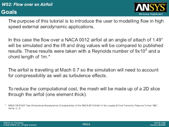
- 2. Goals The purpose of this tutorial is to introduce the user to modelling flow in high
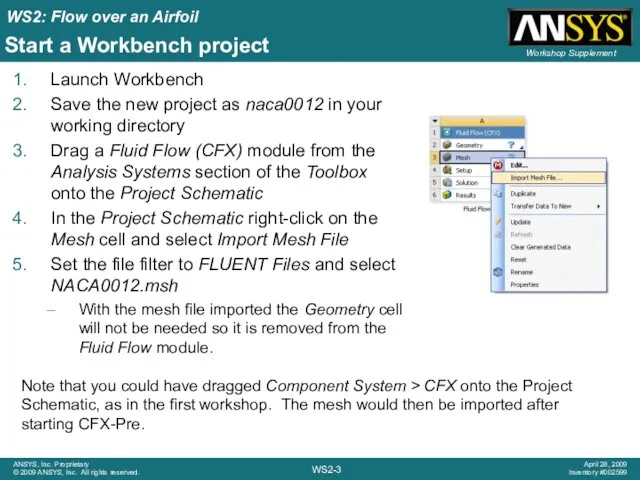
- 3. Start a Workbench project Launch Workbench Save the new project as naca0012 in your working directory
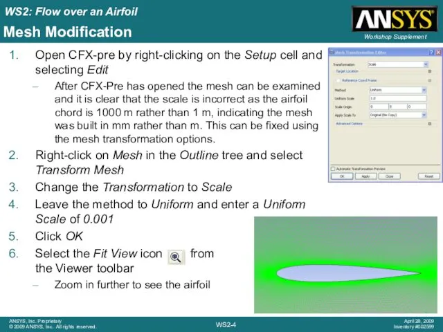
- 4. Mesh Modification Open CFX-pre by right-clicking on the Setup cell and selecting Edit After CFX-Pre has
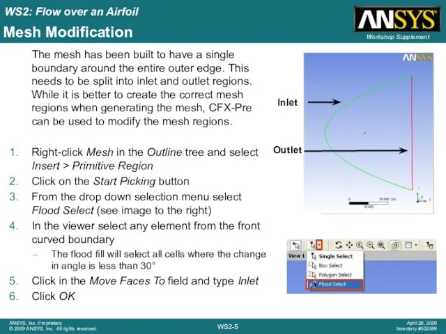
- 5. Mesh Modification The mesh has been built to have a single boundary around the entire outer
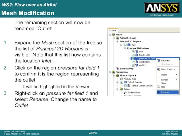
- 6. Mesh Modification The remaining section will now be renamed “Outlet”. Expand the Mesh section of the
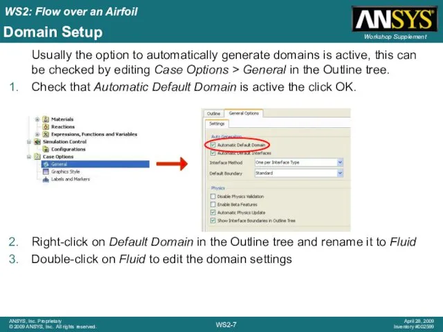
- 7. Domain Setup Usually the option to automatically generate domains is active, this can be checked by
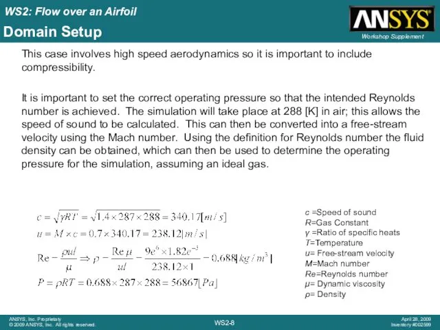
- 8. Domain Setup This case involves high speed aerodynamics so it is important to include compressibility. It
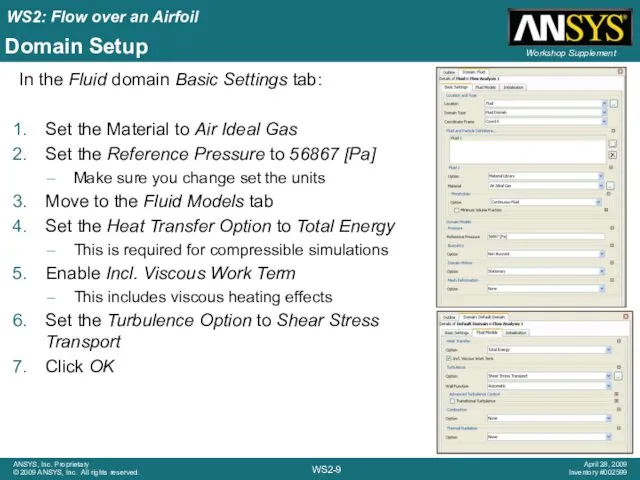
- 9. Domain Setup In the Fluid domain Basic Settings tab: Set the Material to Air Ideal Gas
- 10. Boundary Conditions An outlet relative pressure of 0 [Pa] will now be applied. This pressure is
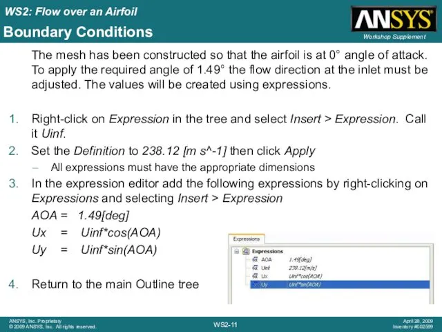
- 11. Boundary Conditions The mesh has been constructed so that the airfoil is at 0° angle of
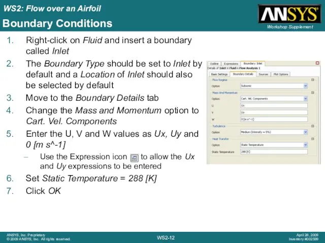
- 12. Boundary Conditions Right-click on Fluid and insert a boundary called Inlet The Boundary Type should be
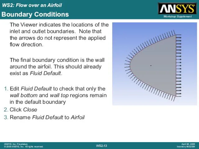
- 13. Boundary Conditions The Viewer indicates the locations of the inlet and outlet boundaries. Note that the
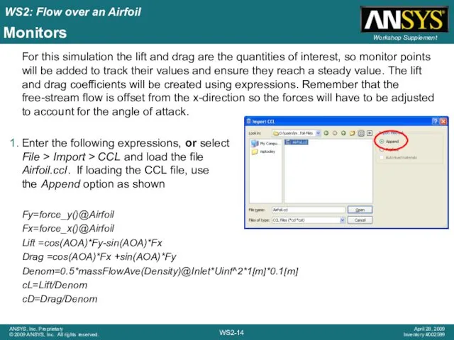
- 14. Monitors For this simulation the lift and drag are the quantities of interest, so monitor points
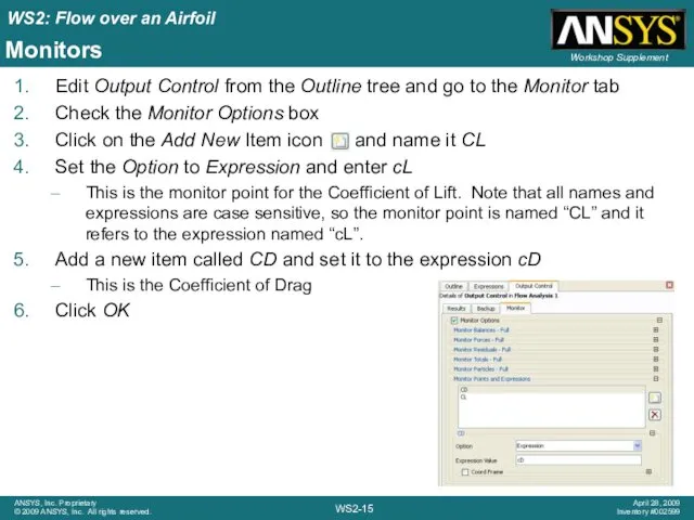
- 15. Monitors Edit Output Control from the Outline tree and go to the Monitor tab Check the
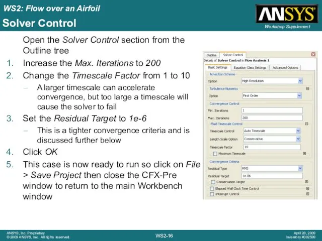
- 16. Solver Control Open the Solver Control section from the Outline tree Increase the Max. Iterations to
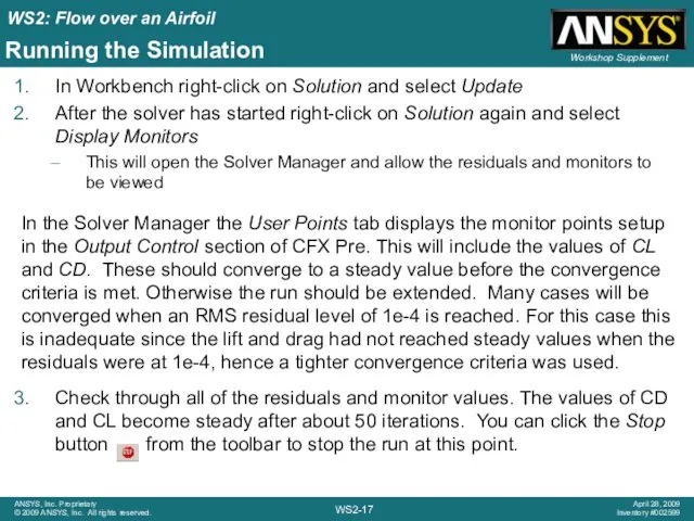
- 17. Running the Simulation In Workbench right-click on Solution and select Update After the solver has started
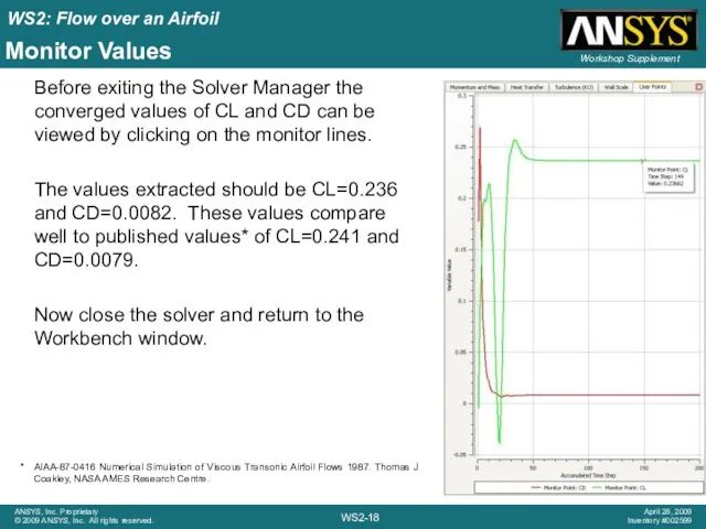
- 18. Monitor Values Before exiting the Solver Manager the converged values of CL and CD can be
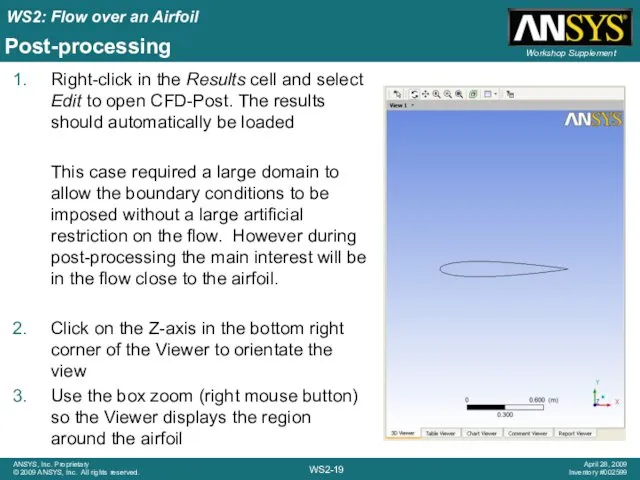
- 19. Post-processing Right-click in the Results cell and select Edit to open CFD-Post. The results should automatically
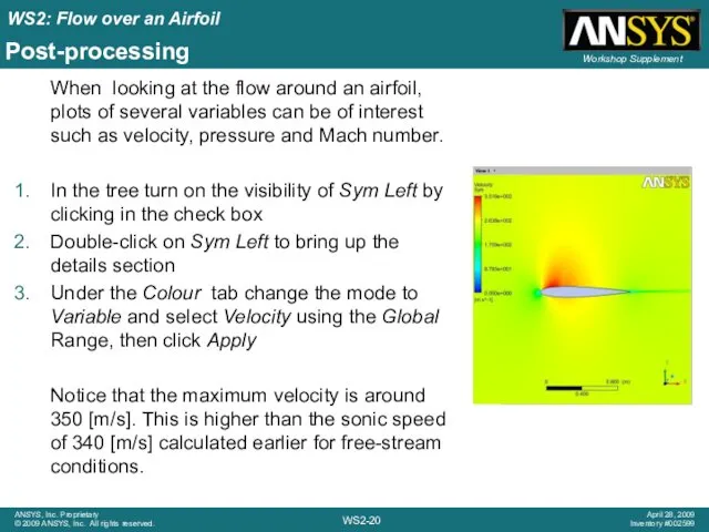
- 20. Post-processing When looking at the flow around an airfoil, plots of several variables can be of
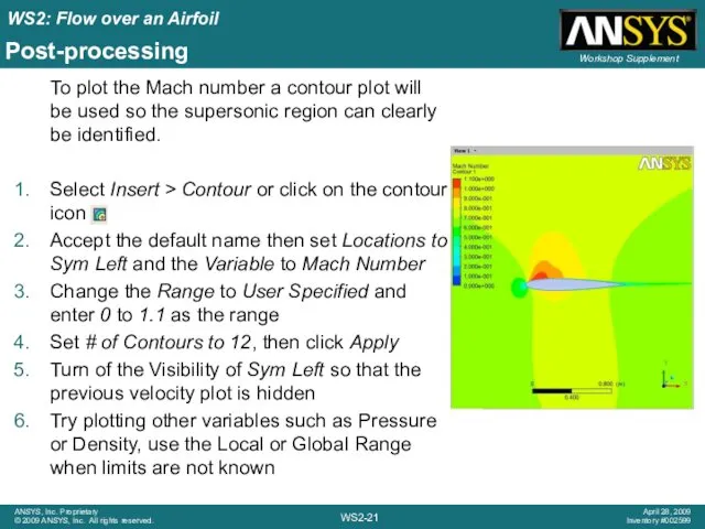
- 21. Post-processing To plot the Mach number a contour plot will be used so the supersonic region
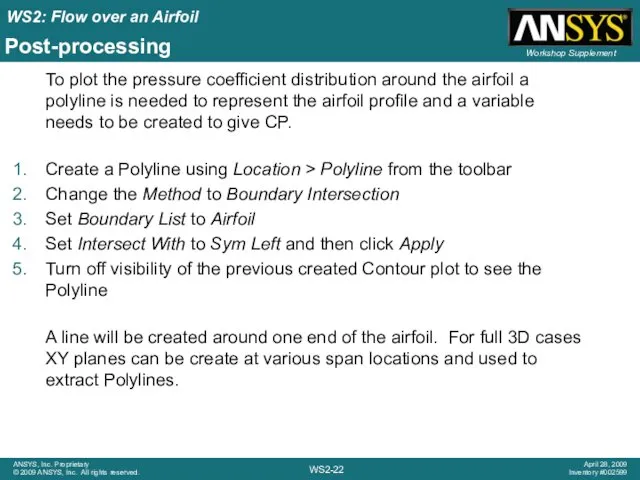
- 22. Post-processing To plot the pressure coefficient distribution around the airfoil a polyline is needed to represent
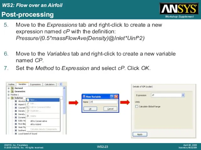
- 23. Post-processing Move to the Expressions tab and right-click to create a new expression named cP with
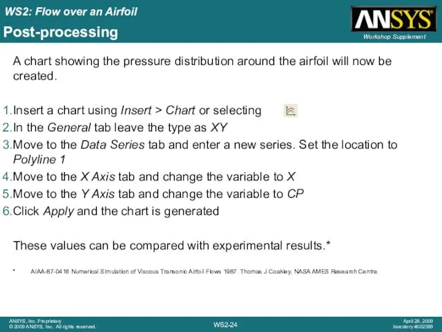
- 24. Post-processing A chart showing the pressure distribution around the airfoil will now be created. Insert a
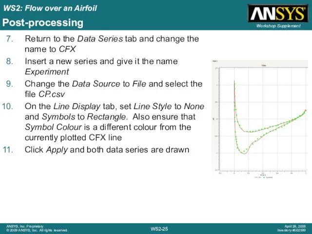
- 25. Post-processing Return to the Data Series tab and change the name to CFX Insert a new
- 26. Summary The workshop has covered: Loading an existing mesh Scaling the mesh Generating New Regions from
- 28. Скачать презентацию
Goals
The purpose of this tutorial is to introduce the user to
Goals
The purpose of this tutorial is to introduce the user to
Start a Workbench project
Launch Workbench
Save the new project as naca0012 in
Start a Workbench project
Launch Workbench
Save the new project as naca0012 in
Mesh Modification
Open CFX-pre by right-clicking on the Setup cell and selecting
Mesh Modification
Open CFX-pre by right-clicking on the Setup cell and selecting
Mesh Modification
The mesh has been built to have a single
Mesh Modification
The mesh has been built to have a single
Mesh Modification
The remaining section will now be renamed “Outlet”.
Expand
Mesh Modification
The remaining section will now be renamed “Outlet”.
Expand
Domain Setup
Usually the option to automatically generate domains is active, this
Domain Setup
Usually the option to automatically generate domains is active, this
Domain Setup
This case involves high speed aerodynamics so it is important
Domain Setup
This case involves high speed aerodynamics so it is important
Domain Setup
In the Fluid domain Basic Settings tab:
Set the Material to
Domain Setup
In the Fluid domain Basic Settings tab:
Set the Material to
![Boundary Conditions An outlet relative pressure of 0 [Pa] will](/_ipx/f_webp&q_80&fit_contain&s_1440x1080/imagesDir/jpg/96060/slide-9.jpg)
Boundary Conditions
An outlet relative pressure of 0 [Pa] will now be
Boundary Conditions
An outlet relative pressure of 0 [Pa] will now be
Boundary Conditions
The mesh has been constructed so that the airfoil
Boundary Conditions
The mesh has been constructed so that the airfoil
Boundary Conditions
Right-click on Fluid and insert a boundary called Inlet
The Boundary
Boundary Conditions
Right-click on Fluid and insert a boundary called Inlet
The Boundary
Boundary Conditions
The Viewer indicates the locations of the inlet and outlet
Boundary Conditions
The Viewer indicates the locations of the inlet and outlet
Monitors
For this simulation the lift and drag are the quantities of
Monitors
For this simulation the lift and drag are the quantities of
Monitors
Edit Output Control from the Outline tree and go to the
Monitors
Edit Output Control from the Outline tree and go to the
Solver Control
Open the Solver Control section from the Outline tree
Increase the
Solver Control
Open the Solver Control section from the Outline tree
Increase the
Running the Simulation
In Workbench right-click on Solution and select Update
After the
Running the Simulation
In Workbench right-click on Solution and select Update
After the
Monitor Values
Before exiting the Solver Manager the converged values of CL
Monitor Values
Before exiting the Solver Manager the converged values of CL
Post-processing
Right-click in the Results cell and select Edit to open CFD-Post.
Post-processing
Right-click in the Results cell and select Edit to open CFD-Post.
Post-processing
When looking at the flow around an airfoil, plots of several
Post-processing
When looking at the flow around an airfoil, plots of several
Post-processing
To plot the Mach number a contour plot will be used
Post-processing
To plot the Mach number a contour plot will be used
Post-processing
To plot the pressure coefficient distribution around the airfoil a polyline
Post-processing
To plot the pressure coefficient distribution around the airfoil a polyline
Post-processing
Move to the Expressions tab and right-click to create a new
Post-processing
Move to the Expressions tab and right-click to create a new
Post-processing
A chart showing the pressure distribution around the airfoil will now
Post-processing
A chart showing the pressure distribution around the airfoil will now
Post-processing
Return to the Data Series tab and change the name to
Post-processing
Return to the Data Series tab and change the name to
Summary
The workshop has covered:
Loading an existing mesh
Scaling the mesh
Generating New Regions
Summary
The workshop has covered:
Loading an existing mesh
Scaling the mesh
Generating New Regions
 Befree. Cons of social networks
 Комплекс заданий по освоению графики
 Как отправить заказ. Инструкция
 Использование информационно-коммуникационных технологий в процессе обучения физике
 Adobe Photoshop графикалық редакторы
 Информатизация общества
 Объектно-ориентированное программирование. Классы в C#
 Государственная политика в сфере формирования электронного правительства
 Вычисление суммы элементов массива. Начала программирования
 3. Java Persistence API. 5. Transaction Management
 Построение и анализ эффективных алгоритмов
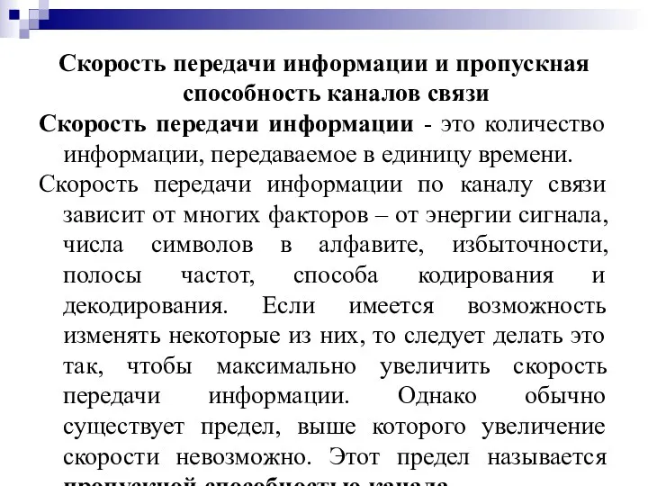 Скорость передачи информации и пропускная способность каналов связи
 Ақпараттық коммуникациялықтехнологияны қолдану негізінде білім сапасын арттыру жолдары
 Основные понятия языка Паскаль
 Правовое регулирование киберпреступности в РФ
 Подготовка к контрольной работе Начала программирования
 Презентация Подходы к понятию информации и измерению информации.
 Бағдарламалық жасақтама
 Текстовый редактор. Возможности и назначение
 Создание анимации. Создание анимации
 Abstractions. Конкретные типы. Абстрактные типы
 Операционные системы. (11 класс)
 Pастровая и векторная графика
 1С:Предприятие 8. Общепит. Презентация отраслевого решения
 Применение компьютерной графики. Цветовые модели
 История развития языка UML
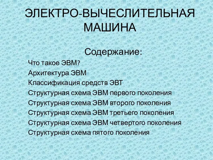 Электро-вычислительная машина
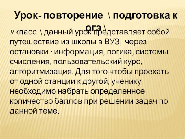 Урок- повторение \ подготовка к ОГЭ\ 9 класс