- Types and basic structures data in R

Содержание
- 2. The purpose of the lecture is to familiarize yourself with the basic data types used in
- 3. 1. Data types in R 2. Basic data structures: 2.1 Vectors 2.2 Matrices 2.3 Arrays 2.4
- 4. Visual statistics. We use R! A. B. Shipunov, E. M. Baldin, P. A. Volkova, A. I.
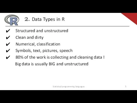
- 5. 2. Data Types in R Structured and unstructured Clean and dirty Numerical, classification Symbols, text, pictures,
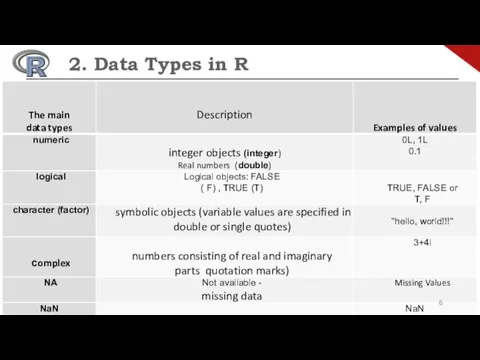
- 6. Statistical programming languages 2. Data Types in R
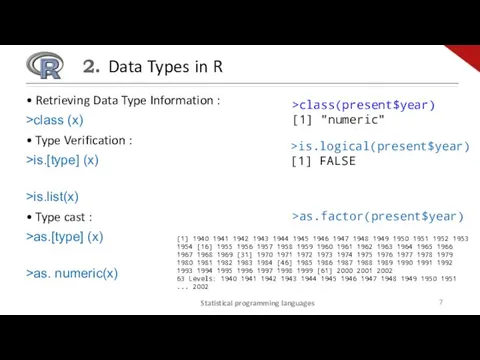
- 7. Statistical programming languages • Retrieving Data Type Information : >class (x) • Type Verification : >is.[type]
- 8. Statistical programming languages MISSING VALUES - NA NA test:: >is.na (x) Getting rid of NA:: >na.omit
- 9. Statistical programming languages 2. Data Types in R nominal continuous ordered discrete Define the data types
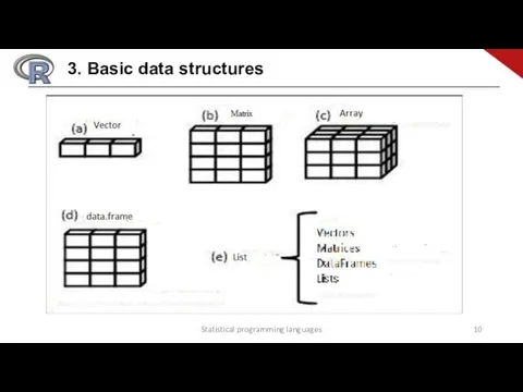
- 10. Statistical programming languages 3. Basic data structures
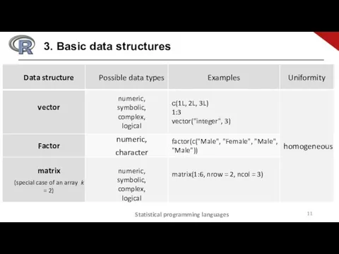
- 11. Statistical programming languages 3. Basic data structures
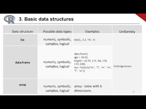
- 12. Statistical programming languages 3. Basic data structures
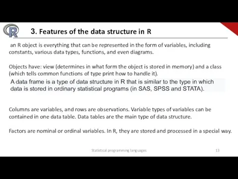
- 13. Statistical programming languages 3. Features of the data structure in R an R object is everything
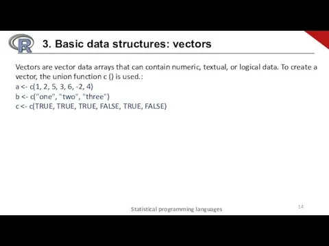
- 14. Statistical programming languages 3. Basic data structures: vectors Vectors are vector data arrays that can contain
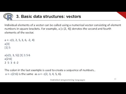
- 15. Statistical programming languages 3. Basic data structures: vectors Individual elements of a vector can be called
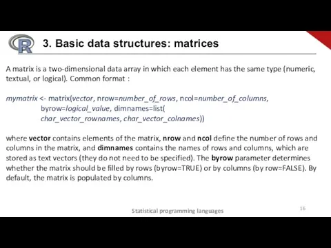
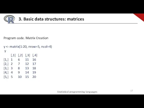
- 16. Statistical programming languages 3. Basic data structures: matrices A matrix is a two-dimensional data array in
- 17. Statistical programming languages 3. Basic data structures: matrices Program code. Matrix Creation y y [,1] [,2]
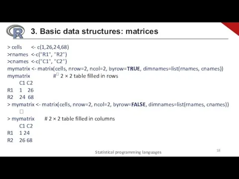
- 18. Statistical programming languages 3. Basic data structures: matrices > cells >rnames >cnames mymatrix mymatrix # 2
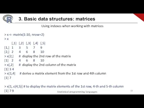
- 19. Statistical programming languages 3. Basic data structures: matrices Using indexes when working with matrices > x
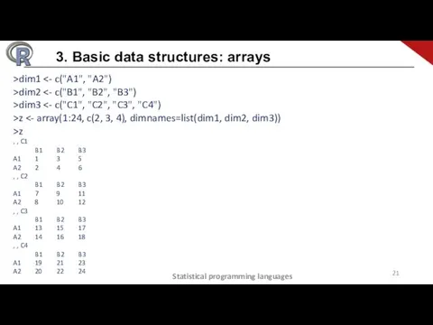
- 20. Statistical programming languages 3. Basic data structures: arrays Arrays are similar to matrices, but can have
- 21. Statistical programming languages 3. Basic data structures: arrays >dim1 >dim2 >dim3 >z >z , , C1
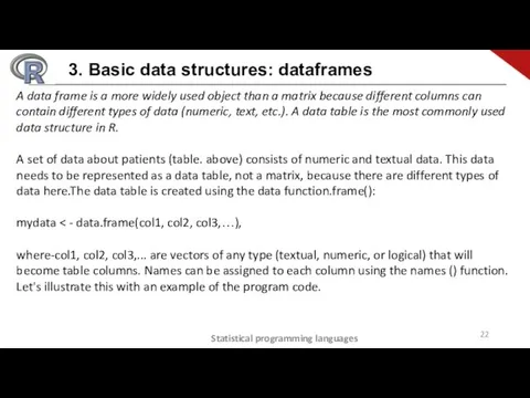
- 22. Statistical programming languages 3. Basic data structures: dataframes A data frame is a more widely used
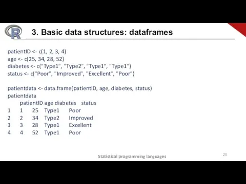
- 23. Statistical programming languages 3. Basic data structures: dataframes patientID age diabetes status patientdata patientdata patientID age
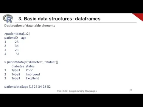
- 24. Statistical programming languages 3. Basic data structures: dataframes Designation of data table elements >patientdata[1:2] patientID age
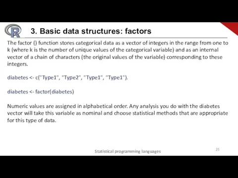
- 25. Statistical programming languages 3. Basic data structures: factors The factor () function stores categorical data as
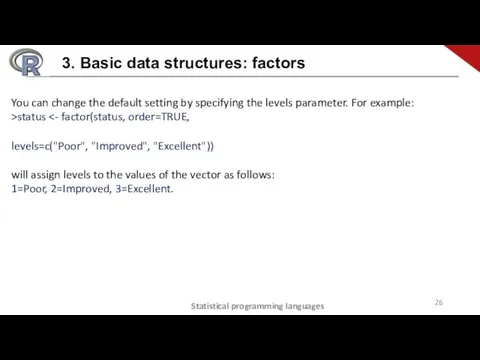
- 26. Statistical programming languages 3. Basic data structures: factors You can change the default setting by specifying
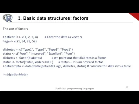
- 27. Statistical programming languages 3. Basic data structures: factors The use of factors >patientID >age diabetes status
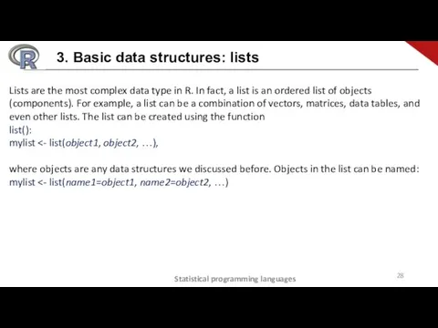
- 28. Statistical programming languages 3. Basic data structures: lists Lists are the most complex data type in
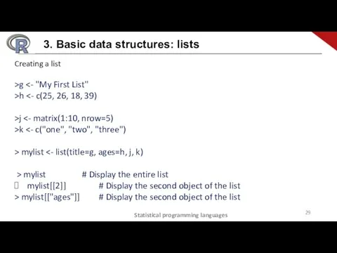
- 29. Statistical programming languages 3. Basic data structures: lists Creating a list >g >h >j >k >
- 31. Скачать презентацию

The purpose of the lecture is to familiarize yourself with the

1. Data types in R
2. Basic data structures:
2.1 Vectors
1. Data types in R
2. Basic data structures:
2.1 Vectors
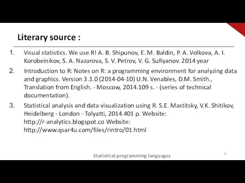
Visual statistics. We use R! A. B. Shipunov, E. M. Baldin,
Visual statistics. We use R! A. B. Shipunov, E. M. Baldin,
2. Data Types in R
Structured and unstructured
Clean and dirty
Numerical,
2. Data Types in R
Structured and unstructured
Clean and dirty
Numerical,
Statistical programming languages
2. Data Types in R
Statistical programming languages
2. Data Types in R
Statistical programming languages
• Retrieving Data Type Information :
>class (x)
• Type Verification
Statistical programming languages
• Retrieving Data Type Information :
>class (x)
• Type Verification
Statistical programming languages
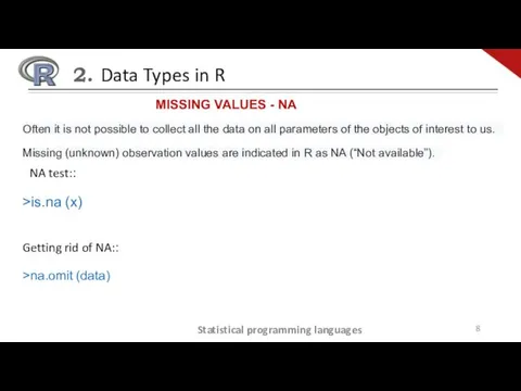
MISSING VALUES - NA
NA test::
>is.na (x)
Getting rid of NA::
Statistical programming languages
MISSING VALUES - NA
NA test::
>is.na (x)
Getting rid of NA::

Statistical programming languages
2. Data Types in R
nominal
continuous
ordered
discrete
Define the data types for
Statistical programming languages
2. Data Types in R
nominal
continuous
ordered
discrete
Define the data types for
Statistical programming languages
3. Basic data structures
Statistical programming languages
3. Basic data structures
Statistical programming languages
3. Basic data structures
Statistical programming languages
3. Basic data structures
Statistical programming languages
3. Basic data structures
Statistical programming languages
3. Basic data structures
Statistical programming languages
3. Features of the data structure in R
an R
Statistical programming languages
3. Features of the data structure in R
an R
Statistical programming languages
3. Basic data structures: vectors
Vectors are vector data arrays
Statistical programming languages
3. Basic data structures: vectors
Vectors are vector data arrays
Statistical programming languages
3. Basic data structures: vectors
Individual elements of a vector
Statistical programming languages
3. Basic data structures: vectors
Individual elements of a vector
Statistical programming languages
3. Basic data structures: matrices
A matrix is a two-dimensional
Statistical programming languages
3. Basic data structures: matrices
A matrix is a two-dimensional
Statistical programming languages
3. Basic data structures: matrices
Program code. Matrix Creation
y <-
Statistical programming languages
3. Basic data structures: matrices
Program code. Matrix Creation
y <-
Statistical programming languages
3. Basic data structures: matrices
> cells <- c(1,26,24,68)
>rnames <-c("R1", "R2")
>cnames <-c("C1", "C2")
mymatrix
Statistical programming languages
3. Basic data structures: matrices
> cells <- c(1,26,24,68)
>rnames <-c("R1", "R2")
>cnames <-c("C1", "C2")
mymatrix
Statistical programming languages
3. Basic data structures: matrices
Using indexes when working with
Statistical programming languages
3. Basic data structures: matrices
Using indexes when working with

Statistical programming languages
3. Basic data structures: arrays
Arrays are similar to matrices,
Statistical programming languages
3. Basic data structures: arrays
Arrays are similar to matrices,
Statistical programming languages
3. Basic data structures: arrays
>dim1 <- c("A1", "A2")
>dim2 <-
Statistical programming languages
3. Basic data structures: arrays
>dim1 <- c("A1", "A2")
>dim2 <-
Statistical programming languages
3. Basic data structures: dataframes
A data frame is a
Statistical programming languages
3. Basic data structures: dataframes
A data frame is a
Statistical programming languages
3. Basic data structures: dataframes
patientID <- c(1, 2, 3,
Statistical programming languages
3. Basic data structures: dataframes
patientID <- c(1, 2, 3,
Statistical programming languages
3. Basic data structures: dataframes
Designation of data table elements
>patientdata[1:2]
Statistical programming languages
3. Basic data structures: dataframes
Designation of data table elements
>patientdata[1:2]
Statistical programming languages
3. Basic data structures: factors
The factor () function stores
Statistical programming languages
3. Basic data structures: factors
The factor () function stores
Statistical programming languages
3. Basic data structures: factors
You can change the default
Statistical programming languages
3. Basic data structures: factors
You can change the default
Statistical programming languages
3. Basic data structures: factors
The use of factors
>patientID <-
Statistical programming languages
3. Basic data structures: factors
The use of factors
>patientID <-
Statistical programming languages
3. Basic data structures: lists
Lists are the most complex
Statistical programming languages
3. Basic data structures: lists
Lists are the most complex
Statistical programming languages
3. Basic data structures: lists
Creating a list
>g <- "My
Statistical programming languages
3. Basic data structures: lists
Creating a list
>g <- "My
 Вестник ХММР №4, июль 2018
 Создание Web-страниц с помощью html-кода
 Системы счисления (проверим знания)
 Локальды компьютерлік желілер. Локальды желілердің түрлері
 Автоматизация технических процессов и производств
 Координатная плоскость. Управление исполнителем Чертежник.
 Взаимодействия с внешними (межведомственное взаимодействие) системами
 Основы операционных систем
 Электронная торговля
 Графічний інтерфейс користувача у мові Python
 Типы, переменные, управляющие инструкции. Ссылочные типы и переменные. (Тема 2.3)
 Моделирование. 9 класс
 Упрощенный приём отправлений (инструкция v.1)
 Bitbucket repository
 Презентация Алгоритм как модель деятельности
 Основы сетей передачи данных. Общие принципы построения сетей. Коммутация каналов и пакетов
 Материалы к уроку информатики Вставка объектов в презентацию
 Создание презентаций в Microsoft Power Point
 Kutubxona faoliyatida elektron ta’lim kontentlarini yaratish
 Связь ассемблера с языками высокого уровня
 Базы данных. Реляционная модель данных
 Создание Telegram-бота
 Системы счисления. Перевод чисел из одной системы счисления в другую систему счисления
 Урок информатики Создание калькулятора с использованием языка программирования Visual Basic
 Команда ветвления
 Операционная система Windows
 Машина Тьюринга
 Особенности использования криптографии и электронной подписи при защите персональных данных