- Strategy and Analysis in Using Net Present Value. Decision Trees

Содержание
- 2. Chapter Outline 8.1 Decision Trees 8.2 Sensitivity Analysis, Scenario Analysis, and Break-Even Analysis 8.3 Monte Carlo
- 3. 8.1 Decision Trees Allow us to graphically represent the alternatives available to us in each period
- 4. Example of Decision Tree Do not study Study finance Squares represent decisions to be made. Circles
- 5. Stewart Pharmaceuticals The Stewart Pharmaceuticals Corporation is considering investing in developing a drug that cures the
- 6. Stewart Pharmaceuticals NPV of Full-Scale Production following Successful Test Note that the NPV is calculated as
- 7. Stewart Pharmaceuticals NPV of Full-Scale Production following Unsuccessful Test Note that the NPV is calculated as
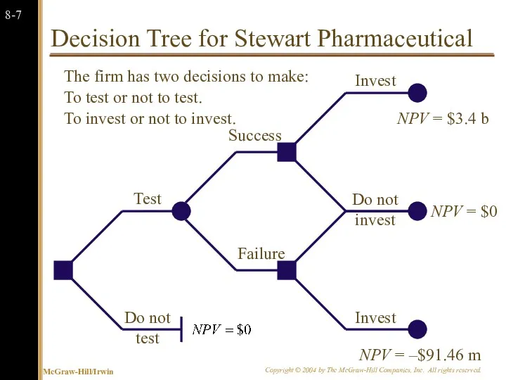
- 8. Decision Tree for Stewart Pharmaceutical Do not test Test Failure Success Do not invest Invest The
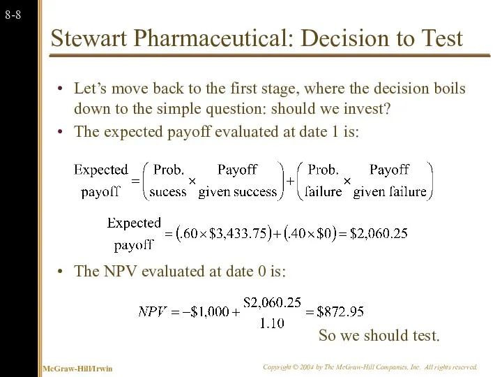
- 9. Stewart Pharmaceutical: Decision to Test Let’s move back to the first stage, where the decision boils
- 10. 8.3 Sensitivity Analysis, Scenario Analysis, and Break-Even Analysis Allows us to look the behind the NPV
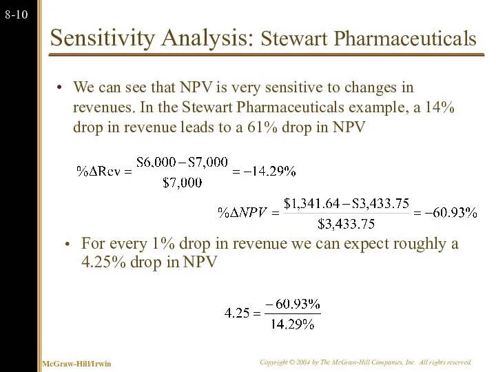
- 11. Sensitivity Analysis: Stewart Pharmaceuticals We can see that NPV is very sensitive to changes in revenues.
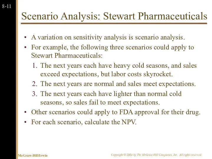
- 12. Scenario Analysis: Stewart Pharmaceuticals A variation on sensitivity analysis is scenario analysis. For example, the following
- 13. Break-Even Analysis: Stewart Pharmaceuticals Another way to examine variability in our forecasts is break-even analysis. In
- 14. Break-Even Analysis: Stewart Pharmaceuticals The project requires an investment of $1,600. In order to cover our
- 15. Break-Even Revenue Stewart Pharmaceuticals Work backwards from OCFBE to Break-Even Revenue Revenue $5,358.72 Variable cost $3,000
- 16. Break-Even Analysis: PBE Now that we have break-even revenue as $5,358.72 million we can calculate break-even
- 17. Break-Even Analysis: Dorm Beds Recall the “Dorm beds” example from the previous chapter. We could be
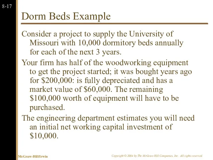
- 18. Dorm Beds Example Consider a project to supply the University of Missouri with 10,000 dormitory beds
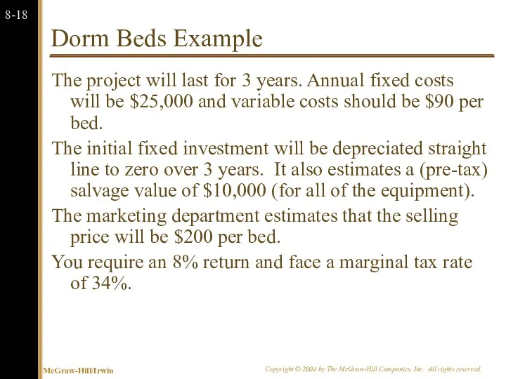
- 19. Dorm Beds Example The project will last for 3 years. Annual fixed costs will be $25,000
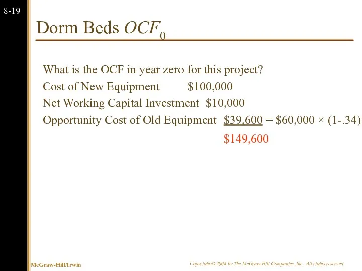
- 20. Dorm Beds OCF0 What is the OCF in year zero for this project? Cost of New
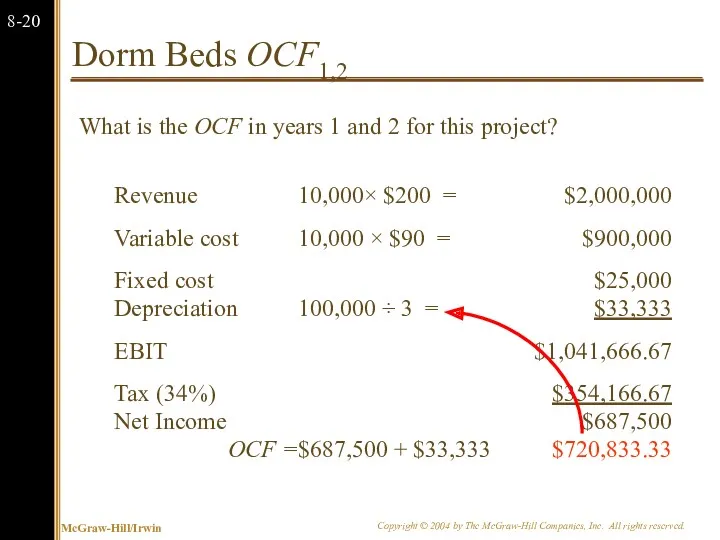
- 21. Dorm Beds OCF1,2 What is the OCF in years 1 and 2 for this project? Revenue
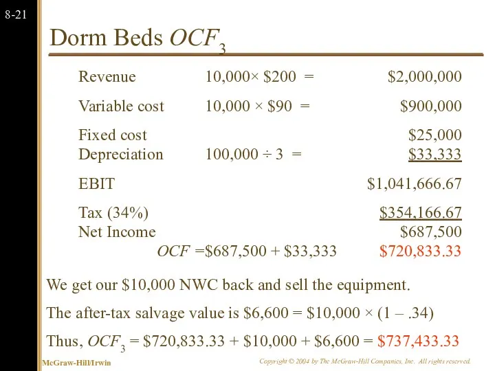
- 22. Dorm Beds OCF3 We get our $10,000 NWC back and sell the equipment. The after-tax salvage
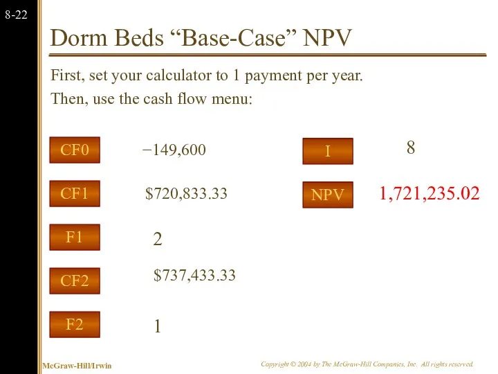
- 23. Dorm Beds “Base-Case” NPV First, set your calculator to 1 payment per year. Then, use the
- 24. Dorm Beds Break-Even Analysis In this example, we should be concerned with break-even price. Let’s start
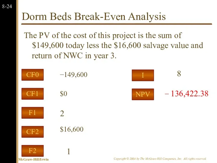
- 25. Dorm Beds Break-Even Analysis The PV of the cost of this project is the sum of
- 26. Break-Even Analysis: OCFBE First, set your calculator to 1 payment per year. PMT I/Y FV PV
- 27. Break-Even Revenue Work backwards from OCFBE to Break-Even Revenue Revenue 10,000× $PBE = $988,035.04 Variable cost
- 28. Break-Even Analysis Now that we have break-even revenue we can calculate break-even price If we sell
- 29. Common Mistake in Break-Even What’s wrong with this line of reasoning? With a price of $200
- 30. Don’t Forget that Variable Cost Varies Revenue QBE × $200 = $88,035.04 + QBE× $110 Variable
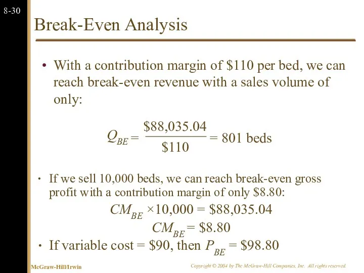
- 31. Break-Even Analysis With a contribution margin of $110 per bed, we can reach break-even revenue with
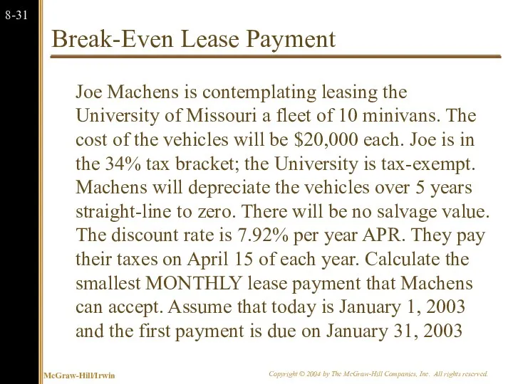
- 32. Break-Even Lease Payment Joe Machens is contemplating leasing the University of Missouri a fleet of 10
- 33. Break-Even Lease Payment: Depreciation Let’s cash flow this out from Joe’s perspective. The operating cash flow
- 34. Present Value of Depreciation Tax Shield The PV of the depreciation tax shields on April 15,
- 35. Present Value of Depreciation Tax Shield The PV of the depreciation tax shields on January 1
- 36. Where we’re at so far: The cars do not cost Joe Machens $200,000. When we consider
- 37. Step Two: Taxes Joe has to pay taxes on last year’s income 1/1/03 1/1/04 1/1/05 1/1/06
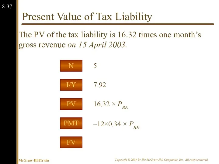
- 38. Present Value of Tax Liability The PV of the tax liability is 16.32 times one month’s
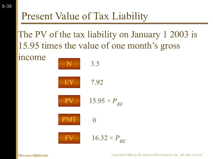
- 39. Present Value of Tax Liability The PV of the tax liability on January 1 2003 is
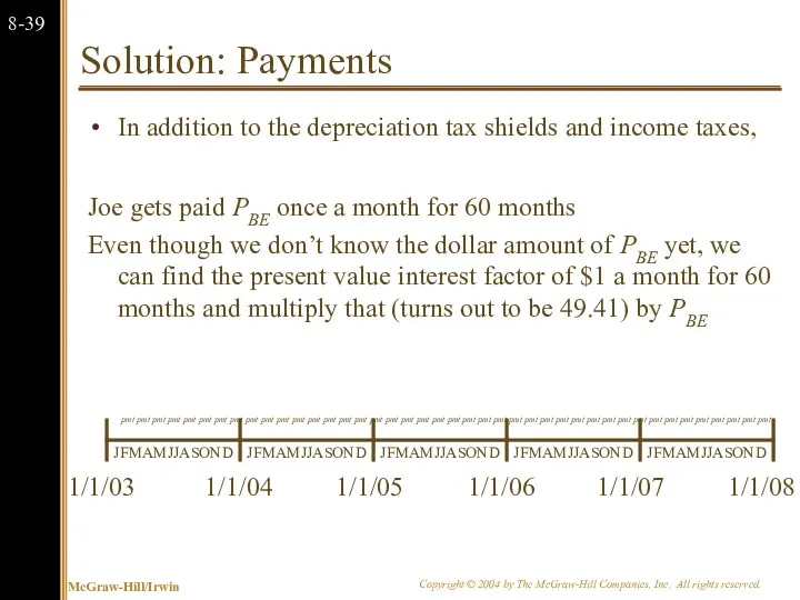
- 40. Solution: Payments In addition to the depreciation tax shields and income taxes, Joe gets paid PBE
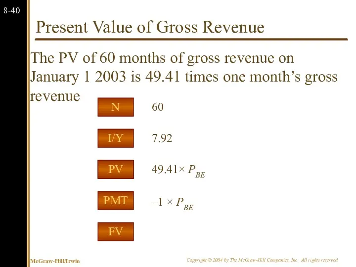
- 41. Present Value of Gross Revenue The PV of 60 months of gross revenue on January 1
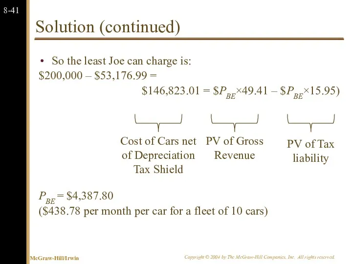
- 42. Solution (continued) So the least Joe can charge is: $200,000 – $53,176.99 = $146,823.01 = $PBE×49.41
- 43. Summary Joe Machens This problem was a bit more complicated than previous problems because of the
- 44. 8.3 Monte Carlo Simulation Monte Carlo simulation is a further attempt to model real-world uncertainty. This
- 45. 8.3 Monte Carlo Simulation Imagine a serious blackjack player who wants to know if he should
- 46. 8.3 Monte Carlo Simulation Monte Carlo simulation of capital budgeting projects is often viewed as a
- 47. 8.4 Options One of the fundamental insights of modern finance theory is that options have value.
- 48. Options The Option to Expand Has value if demand turns out to be higher than expected.
- 49. The Option to Expand Imagine a start-up firm, Campusteria, Inc. which plans to open private (for-profit)
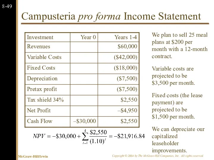
- 50. Campusteria pro forma Income Statement We plan to sell 25 meal plans at $200 per month
- 51. The Option to Expand: Valuing a Start-Up Note that while the Campusteria test site has a
- 52. Discounted Cash Flows and Options We can calculate the market value of a project as the
- 53. The Option to Abandon: Example Suppose that we are drilling an oil well. The drilling rig
- 54. The Option to Abandon: Example Traditional NPV analysis would indicate rejection of the project.
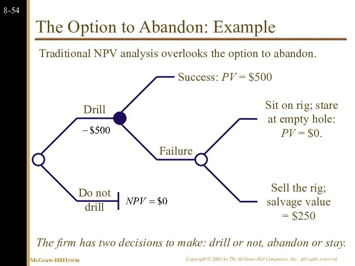
- 55. The Option to Abandon: Example The firm has two decisions to make: drill or not, abandon
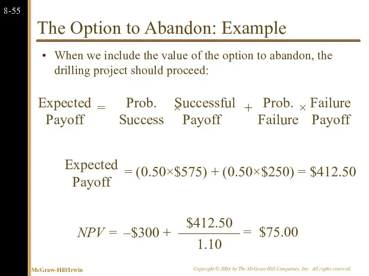
- 56. The Option to Abandon: Example When we include the value of the option to abandon, the
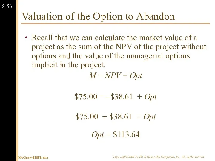
- 57. Valuation of the Option to Abandon Recall that we can calculate the market value of a
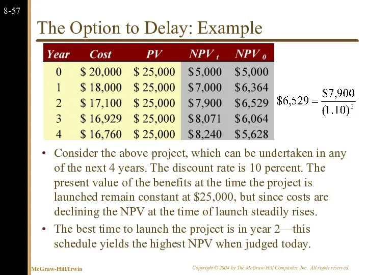
- 58. The Option to Delay: Example Consider the above project, which can be undertaken in any of
- 60. Скачать презентацию
Chapter Outline
8.1 Decision Trees
8.2 Sensitivity Analysis, Scenario Analysis, and
Break-Even
Chapter Outline
8.1 Decision Trees
8.2 Sensitivity Analysis, Scenario Analysis, and
Break-Even
8.1 Decision Trees
Allow us to graphically represent the alternatives available to
8.1 Decision Trees
Allow us to graphically represent the alternatives available to
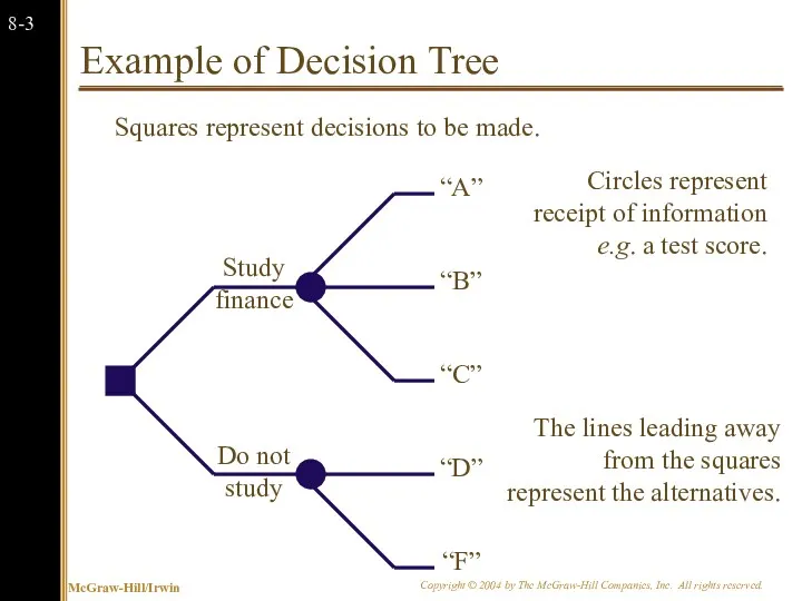
Example of Decision Tree
Do not study
Study finance
Squares represent decisions to be
Example of Decision Tree
Do not study
Study finance
Squares represent decisions to be
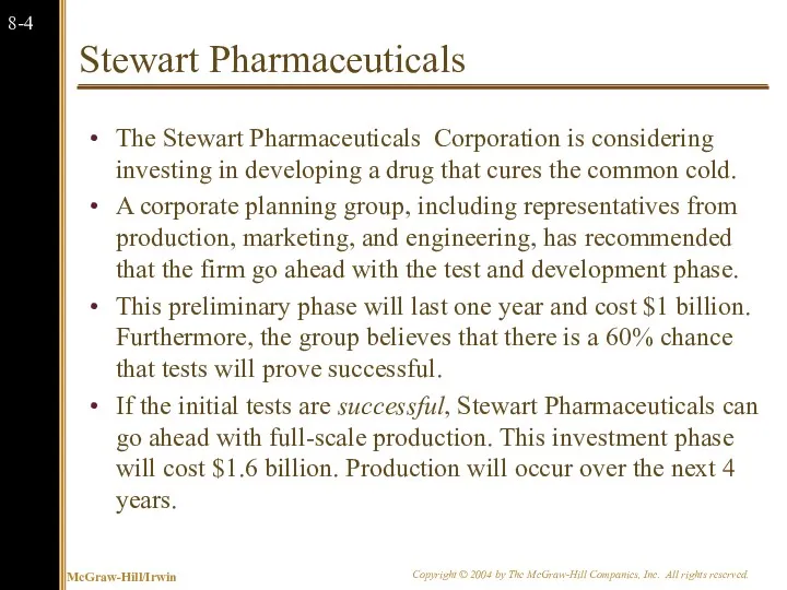
Stewart Pharmaceuticals
The Stewart Pharmaceuticals Corporation is considering investing in developing
Stewart Pharmaceuticals
The Stewart Pharmaceuticals Corporation is considering investing in developing
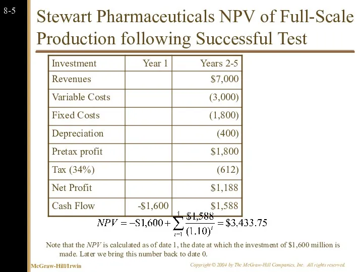
Stewart Pharmaceuticals NPV of Full-Scale Production following Successful Test
Note that the
Stewart Pharmaceuticals NPV of Full-Scale Production following Successful Test
Note that the
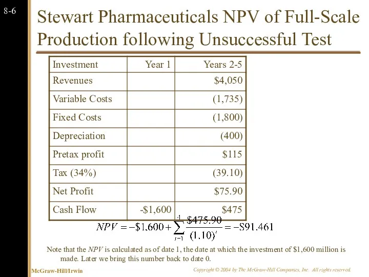
Stewart Pharmaceuticals NPV of Full-Scale Production following Unsuccessful Test
Note that the
Stewart Pharmaceuticals NPV of Full-Scale Production following Unsuccessful Test
Note that the
Decision Tree for Stewart Pharmaceutical
Do not test
Test
Failure
Success
Do not invest
Invest
The firm has
Decision Tree for Stewart Pharmaceutical
Do not test
Test
Failure
Success
Do not invest
Invest
The firm has
Stewart Pharmaceutical: Decision to Test
Let’s move back to the first stage,
Stewart Pharmaceutical: Decision to Test
Let’s move back to the first stage,
8.3 Sensitivity Analysis, Scenario Analysis, and Break-Even Analysis
Allows us to look
8.3 Sensitivity Analysis, Scenario Analysis, and Break-Even Analysis
Allows us to look
Sensitivity Analysis: Stewart Pharmaceuticals
We can see that NPV is very
Sensitivity Analysis: Stewart Pharmaceuticals
We can see that NPV is very
Scenario Analysis: Stewart Pharmaceuticals
A variation on sensitivity analysis is scenario
Scenario Analysis: Stewart Pharmaceuticals
A variation on sensitivity analysis is scenario
Break-Even Analysis: Stewart Pharmaceuticals
Another way to examine variability in our
Break-Even Analysis: Stewart Pharmaceuticals
Another way to examine variability in our
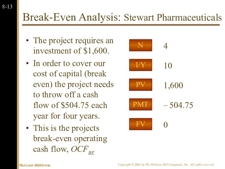
Break-Even Analysis: Stewart Pharmaceuticals
The project requires an investment of $1,600.
In
Break-Even Analysis: Stewart Pharmaceuticals
The project requires an investment of $1,600.
In
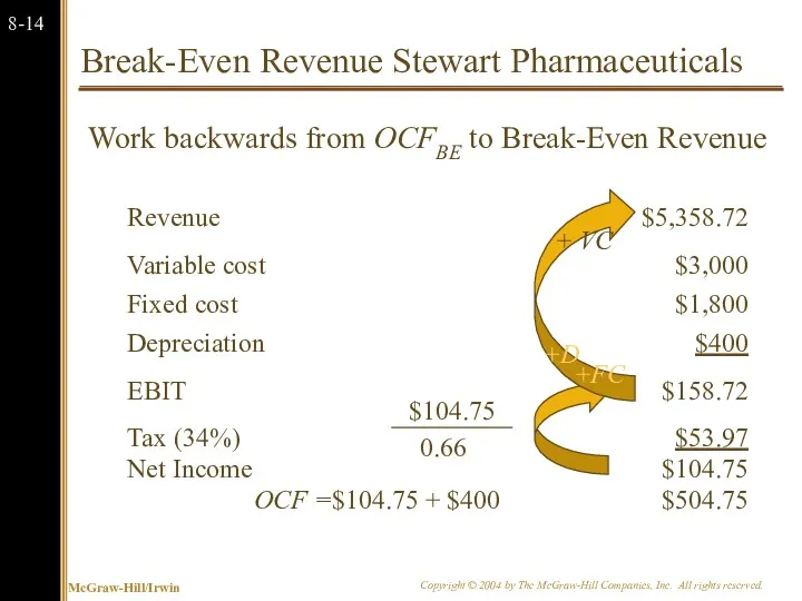
Break-Even Revenue Stewart Pharmaceuticals
Work backwards from OCFBE to Break-Even Revenue
Revenue
$5,358.72
Variable
Break-Even Revenue Stewart Pharmaceuticals
Work backwards from OCFBE to Break-Even Revenue
Revenue
$5,358.72
Variable
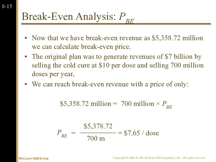
Break-Even Analysis: PBE
Now that we have break-even revenue as $5,358.72 million
Break-Even Analysis: PBE
Now that we have break-even revenue as $5,358.72 million
Break-Even Analysis: Dorm Beds
Recall the “Dorm beds” example from the previous
Break-Even Analysis: Dorm Beds
Recall the “Dorm beds” example from the previous
Dorm Beds Example
Consider a project to supply the University of Missouri
Dorm Beds Example
Consider a project to supply the University of Missouri
Dorm Beds Example
The project will last for 3 years. Annual fixed
Dorm Beds Example
The project will last for 3 years. Annual fixed
Dorm Beds OCF0
What is the OCF in year zero for this
Dorm Beds OCF0
What is the OCF in year zero for this
Dorm Beds OCF1,2
What is the OCF in years 1 and 2
Dorm Beds OCF1,2
What is the OCF in years 1 and 2
Dorm Beds OCF3
We get our $10,000 NWC back and sell the
Dorm Beds OCF3
We get our $10,000 NWC back and sell the
Dorm Beds “Base-Case” NPV
First, set your calculator to 1 payment per
Dorm Beds “Base-Case” NPV
First, set your calculator to 1 payment per
Dorm Beds Break-Even Analysis
In this example, we should be concerned with
Dorm Beds Break-Even Analysis
In this example, we should be concerned with
Dorm Beds Break-Even Analysis
The PV of the cost of this project
Dorm Beds Break-Even Analysis
The PV of the cost of this project
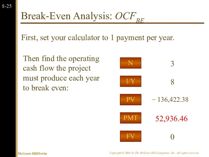
Break-Even Analysis: OCFBE
First, set your calculator to 1 payment per year.
Break-Even Analysis: OCFBE
First, set your calculator to 1 payment per year.
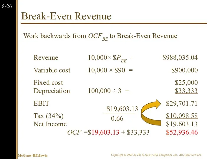
Break-Even Revenue
Work backwards from OCFBE to Break-Even Revenue
Revenue
10,000× $PBE =
$988,035.04
Variable
Break-Even Revenue
Work backwards from OCFBE to Break-Even Revenue
Revenue
10,000× $PBE =
$988,035.04
Variable
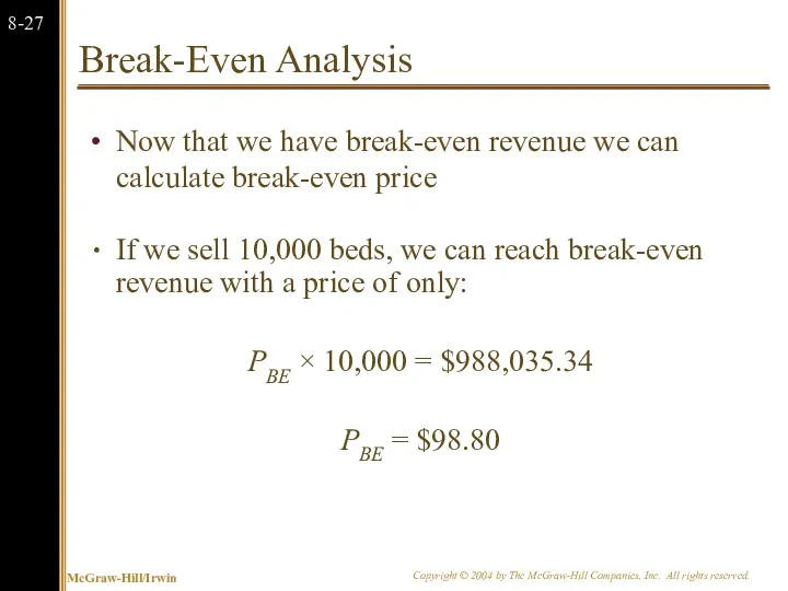
Break-Even Analysis
Now that we have break-even revenue we can calculate break-even
Break-Even Analysis
Now that we have break-even revenue we can calculate break-even
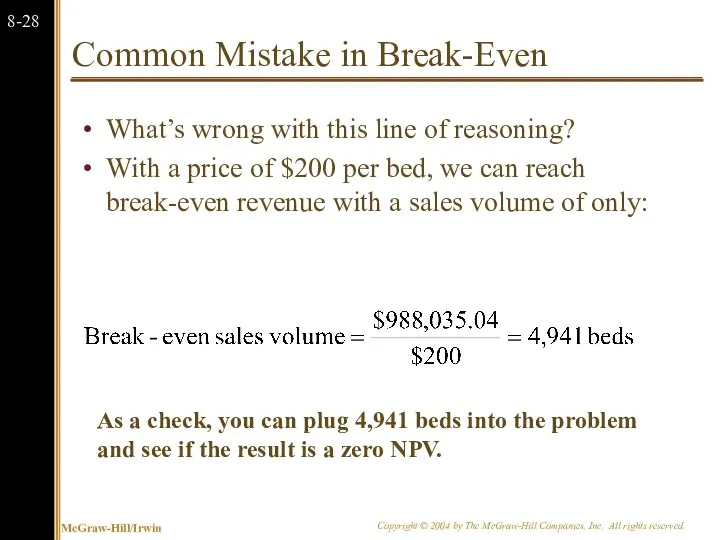
Common Mistake in Break-Even
What’s wrong with this line of reasoning?
With a
Common Mistake in Break-Even
What’s wrong with this line of reasoning?
With a
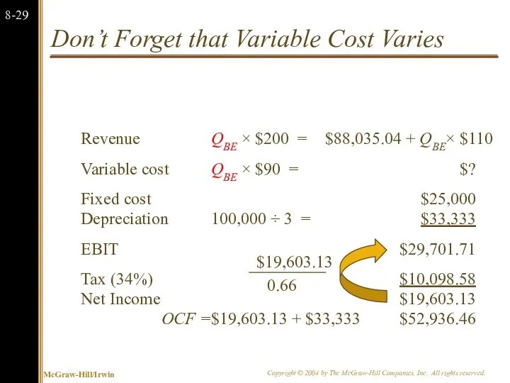
Don’t Forget that Variable Cost Varies
Revenue
QBE × $200 =
$88,035.04 +
Don’t Forget that Variable Cost Varies
Revenue
QBE × $200 =
$88,035.04 +
Break-Even Analysis
With a contribution margin of $110 per bed, we can
Break-Even Analysis
With a contribution margin of $110 per bed, we can
Break-Even Lease Payment
Joe Machens is contemplating leasing the University of Missouri
Break-Even Lease Payment
Joe Machens is contemplating leasing the University of Missouri
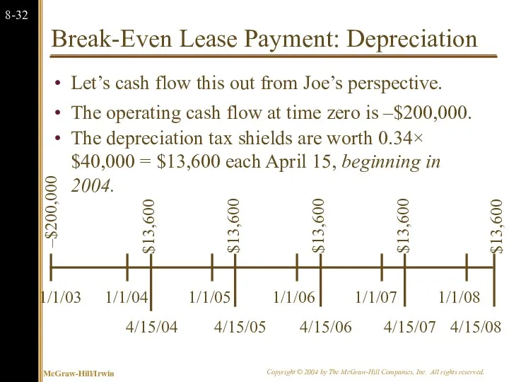
Break-Even Lease Payment: Depreciation
Let’s cash flow this out from Joe’s perspective.
The
Break-Even Lease Payment: Depreciation
Let’s cash flow this out from Joe’s perspective.
The
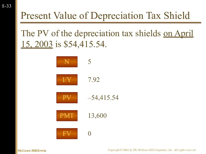
Present Value of Depreciation Tax Shield
The PV of the depreciation tax
Present Value of Depreciation Tax Shield
The PV of the depreciation tax
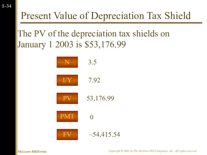
Present Value of Depreciation Tax Shield
The PV of the depreciation tax
Present Value of Depreciation Tax Shield
The PV of the depreciation tax
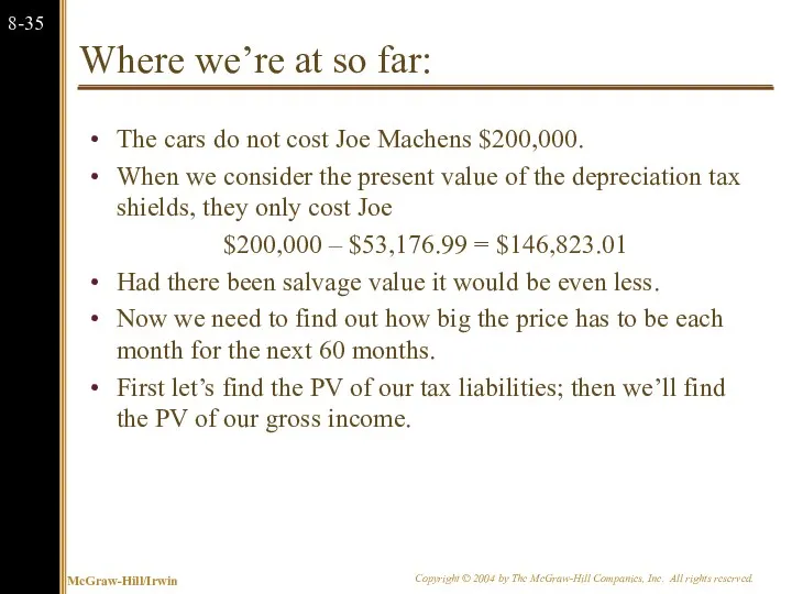
Where we’re at so far:
The cars do not cost Joe Machens
Where we’re at so far:
The cars do not cost Joe Machens
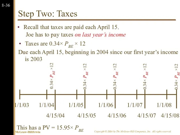
Step Two: Taxes
Joe has to pay taxes on last year’s income
1/1/03
1/1/04
1/1/05
1/1/06
1/1/07
1/1/08
Taxes
Step Two: Taxes
Joe has to pay taxes on last year’s income
1/1/03
1/1/04
1/1/05
1/1/06
1/1/07
1/1/08
Taxes
Present Value of Tax Liability
The PV of the tax liability is
Present Value of Tax Liability
The PV of the tax liability is
Present Value of Tax Liability
The PV of the tax liability on
Present Value of Tax Liability
The PV of the tax liability on
Solution: Payments
In addition to the depreciation tax shields and income taxes,
Solution: Payments
In addition to the depreciation tax shields and income taxes,
Present Value of Gross Revenue
The PV of 60 months of gross
Present Value of Gross Revenue
The PV of 60 months of gross
Solution (continued)
So the least Joe can charge is:
$200,000 – $53,176.99
Solution (continued)
So the least Joe can charge is:
$200,000 – $53,176.99
Summary Joe Machens
This problem was a bit more complicated than previous
Summary Joe Machens
This problem was a bit more complicated than previous
8.3 Monte Carlo Simulation
Monte Carlo simulation is a further attempt to
8.3 Monte Carlo Simulation
Monte Carlo simulation is a further attempt to
8.3 Monte Carlo Simulation
Imagine a serious blackjack player who wants to
8.3 Monte Carlo Simulation
Imagine a serious blackjack player who wants to
8.3 Monte Carlo Simulation
Monte Carlo simulation of capital budgeting projects is
8.3 Monte Carlo Simulation
Monte Carlo simulation of capital budgeting projects is
8.4 Options
One of the fundamental insights of modern finance theory is
8.4 Options
One of the fundamental insights of modern finance theory is
Options
The Option to Expand
Has value if demand turns out to be
Options
The Option to Expand
Has value if demand turns out to be
The Option to Expand
Imagine a start-up firm, Campusteria, Inc. which plans
The Option to Expand
Imagine a start-up firm, Campusteria, Inc. which plans
Campusteria pro forma Income Statement
We plan to sell 25 meal plans
Campusteria pro forma Income Statement
We plan to sell 25 meal plans
The Option to Expand: Valuing a Start-Up
Note that while the Campusteria
The Option to Expand: Valuing a Start-Up
Note that while the Campusteria
Discounted Cash Flows and Options
We can calculate the market value of
Discounted Cash Flows and Options
We can calculate the market value of
The Option to Abandon: Example
Suppose that we are drilling an oil
The Option to Abandon: Example
Suppose that we are drilling an oil
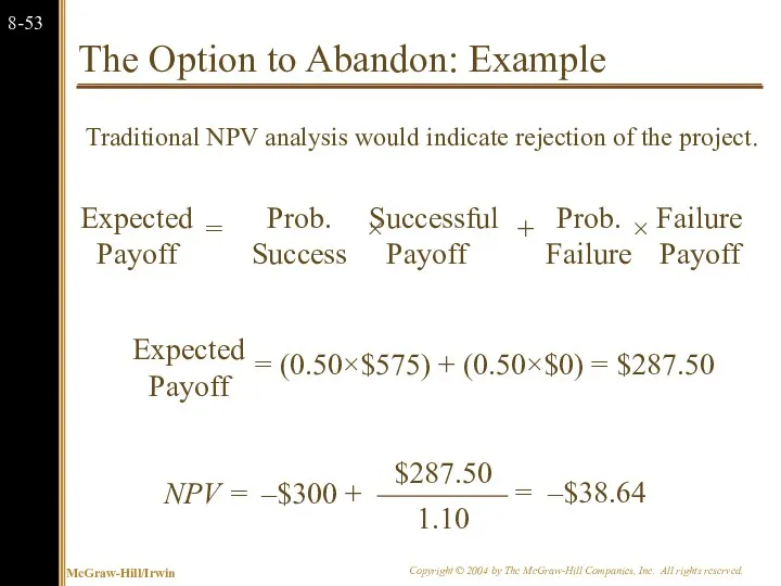
The Option to Abandon: Example
Traditional NPV analysis would indicate rejection
The Option to Abandon: Example
Traditional NPV analysis would indicate rejection
The Option to Abandon: Example
The firm has two decisions to make:
The Option to Abandon: Example
The firm has two decisions to make:
The Option to Abandon: Example
When we include the value of
The Option to Abandon: Example
When we include the value of
Valuation of the Option to Abandon
Recall that we can calculate the
Valuation of the Option to Abandon
Recall that we can calculate the
The Option to Delay: Example
Consider the above project, which can be
The Option to Delay: Example
Consider the above project, which can be
 Акция! 20+1 мотивация оптовых клиентов на закупку кофейных напитков 3в1
 Vodafone PPM booklet
 Компания Atomy
 2018 GRO GLOBAL. Здоровый сон младенца
 Применение средств и методов поведенческой экономики в маркетинговой деятельности туристического предприятия
 Project: Global Social Media Plan // May Topic: Cornering Light Format: Film Date: date related
 Маркетинговые исследования
 ООО “Рус Клин Компани”, бренд Эко Сити Лайф
 Brand Introduction. PART Market Competitiveness
 Подготовка к экзамену. WebPromo Experts
 Product concepts
 Развитие социальной рекламы на телевидении в России
 Зимний уход за кожей лица. АРГО
 Техника продаж. Работа с возражениями
 Помещение (147 м2) в аренду. Характеристика помещения
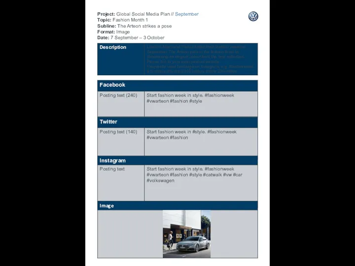 Project: Global Social Media Plan // September Topic: Fashion Month 1 Subline: The Arteon strikes a pose Format: Image
 Коммерческое предложение по размещению рекламы в лифтах г. Электросталь, г. Ногинск
 Маркетинговые коммуникации
 Виртуальная АТС
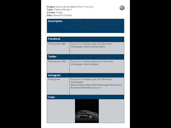 Project: Global Social Media Plan // February Topic: Fashion Shows 1 Format: image Date: Seasonal Content
 Презентация продукта торговый эквайринг
 Adversting
 Марка одежды Сomme des garcons
 Этапы работы над рекламным проектом в стиле шоу
 Экспертное продвижение в INSTAGRAM. Обеспечим рост продаж вашему бизнесу
 Создание собственных онлайн-курсов
 Оптовые поставки детской обуви. ООО АНАЛИТИКА
 Электронная коммерция в Интернете