- Ch8: Hypothesis Testing (2 Samples)

Содержание
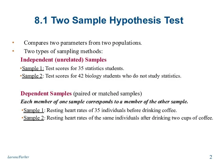
- 2. 8.1 Two Sample Hypothesis Test Compares two parameters from two populations. Two types of sampling methods:
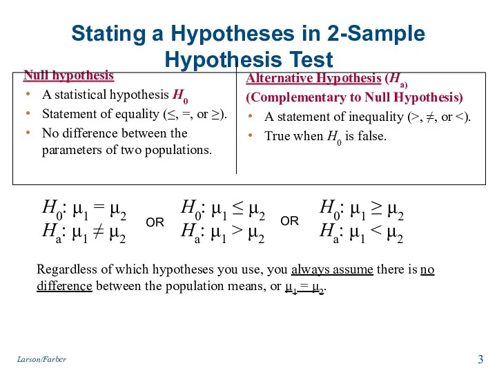
- 3. Stating a Hypotheses in 2-Sample Hypothesis Test Null hypothesis A statistical hypothesis H0 Statement of equality
- 4. Two Sample z-Test for the Difference Between Means (μ1 and μ2.) Three conditions are necessary The
- 5. Using a Two-Sample z-Test for the Difference Between Means (Independent Samples σ1 and σ2 known or
- 6. Example1: Two-Sample z-Test for the Difference Between Means A consumer education organization claims that there is
- 7. Example2: Using Technology to Perform a Two-Sample z-Test The American Automobile Association claims that the average
- 8. 8.2 Two Sample t-Test for the Difference Between Means (σ1 or σ2 unknown) If (σ1 or
- 9. The standard error for the sampling distribution of is Two Sample t-Test for the Difference Between
- 10. Normal or t-Distribution? .
- 11. Two-Sample t-Test for the Difference Between Means - Independent Samples (σ1 or σ2 unknown) State the
- 12. Example: Two-Sample t-Test for the Difference Between Means The braking distances of 8 Volkswagen GTIs and
- 13. Example: Two-Sample t-Test for the Difference Between Means A manufacturer claims that the calling range (in
- 14. The test statistic is the mean of these differences. 8.3 t-Test for the Difference Between Means
- 15. Symbols used for the t-Test for μd The number of pairs of data The difference between
- 16. t-Test for the Difference Between Means (Dependent Samples) State the claim mathematically. Identify the null and
- 17. Example: t-Test for the Difference Between Means A golf club manufacturer claims that golfers can lower
- 18. Solution: Two-Sample t-Test for the Difference Between Means d = (old score) – (new score) Larson/Farber
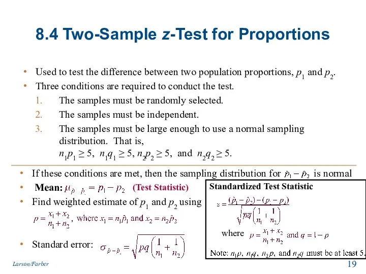
- 19. 8.4 Two-Sample z-Test for Proportions Used to test the difference between two population proportions, p1 and
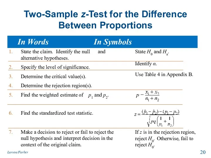
- 20. Two-Sample z-Test for the Difference Between Proportions State the claim. Identify the null and alternative hypotheses.
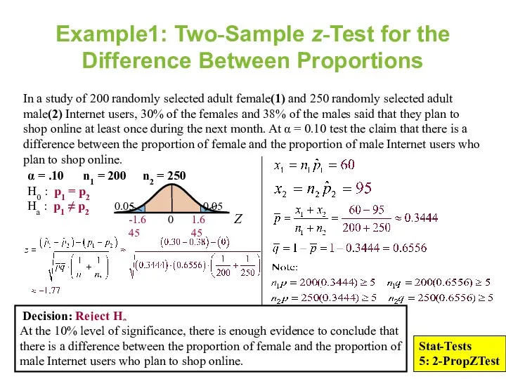
- 21. Example1: Two-Sample z-Test for the Difference Between Proportions In a study of 200 randomly selected adult
- 23. Скачать презентацию
8.1 Two Sample Hypothesis Test
Compares two parameters from two populations.
Two types
8.1 Two Sample Hypothesis Test
Compares two parameters from two populations.
Two types
Stating a Hypotheses in 2-Sample Hypothesis Test
Null hypothesis
A statistical hypothesis
Stating a Hypotheses in 2-Sample Hypothesis Test
Null hypothesis
A statistical hypothesis
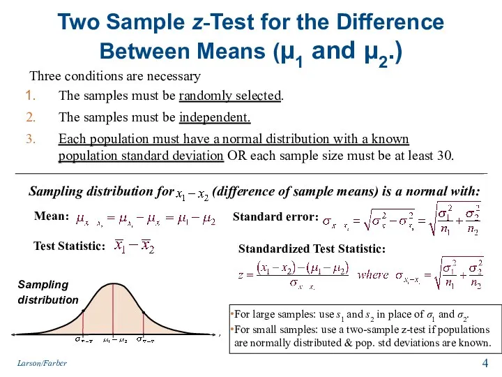
Two Sample z-Test for the Difference Between Means (μ1 and μ2.)
Three
Two Sample z-Test for the Difference Between Means (μ1 and μ2.)
Three
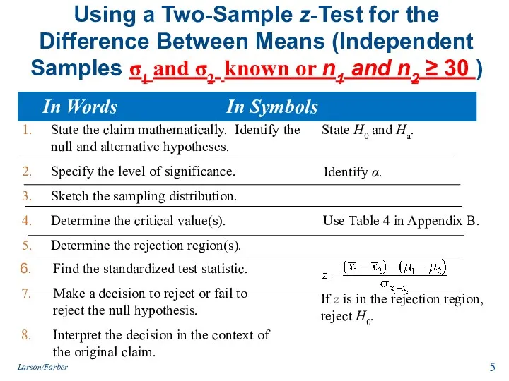
Using a Two-Sample z-Test for the Difference Between Means (Independent Samples
Using a Two-Sample z-Test for the Difference Between Means (Independent Samples
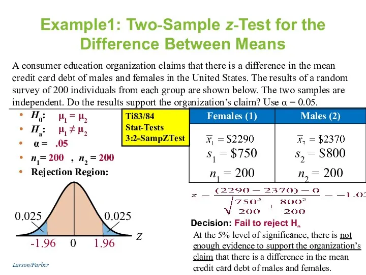
Example1: Two-Sample z-Test for the Difference Between Means
A consumer education organization
Example1: Two-Sample z-Test for the Difference Between Means
A consumer education organization
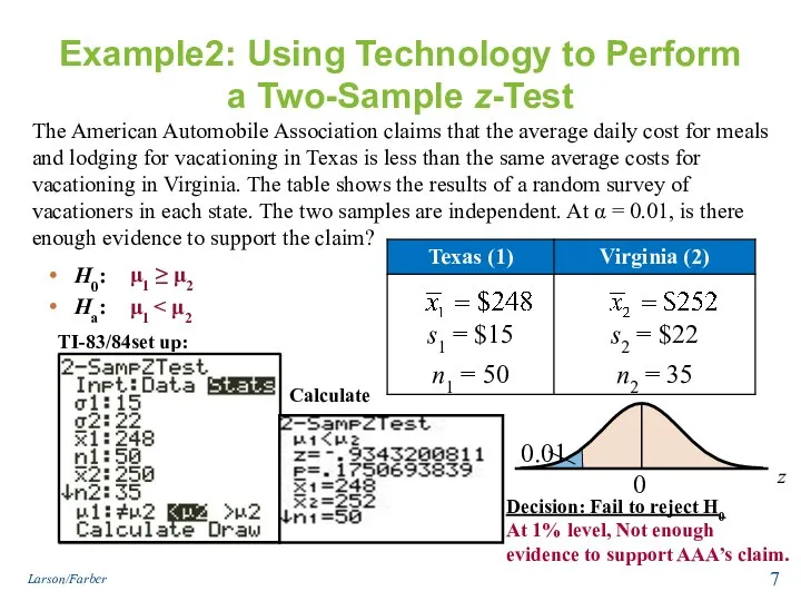
Example2: Using Technology to Perform a Two-Sample z-Test
The American Automobile Association
Example2: Using Technology to Perform a Two-Sample z-Test
The American Automobile Association
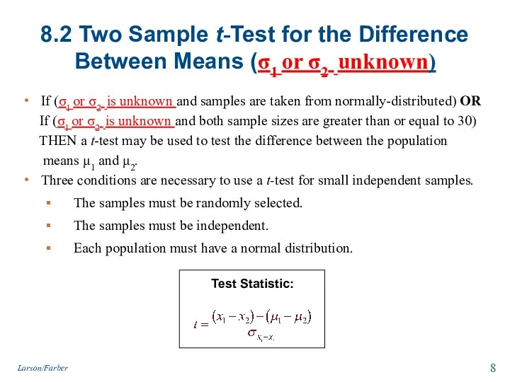
8.2 Two Sample t-Test for the Difference Between Means (σ1 or
8.2 Two Sample t-Test for the Difference Between Means (σ1 or
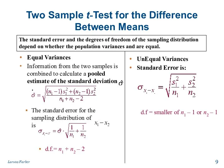
The standard error for the sampling distribution of is
Two Sample
The standard error for the sampling distribution of is
Two Sample
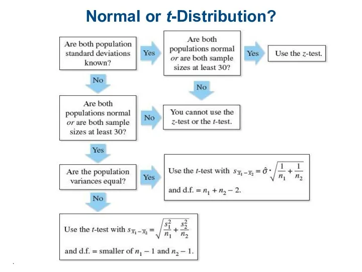
Normal or t-Distribution?
.
Normal or t-Distribution?
.
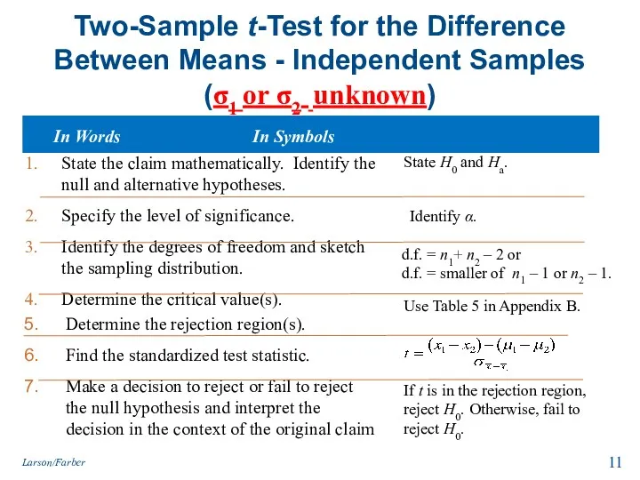
Two-Sample t-Test for the Difference Between Means - Independent Samples
(σ1
Two-Sample t-Test for the Difference Between Means - Independent Samples (σ1
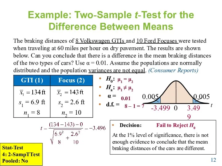
Example: Two-Sample t-Test for the Difference Between Means
The braking distances of
Example: Two-Sample t-Test for the Difference Between Means
The braking distances of

Example: Two-Sample t-Test for the Difference Between Means
A manufacturer claims that
Example: Two-Sample t-Test for the Difference Between Means
A manufacturer claims that
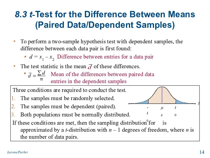
The test statistic is the mean of these differences.
8.3 t-Test for
The test statistic is the mean of these differences.
8.3 t-Test for
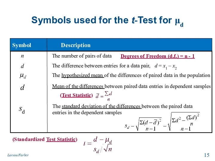
Symbols used for the t-Test for μd
The number of pairs of
Symbols used for the t-Test for μd
The number of pairs of
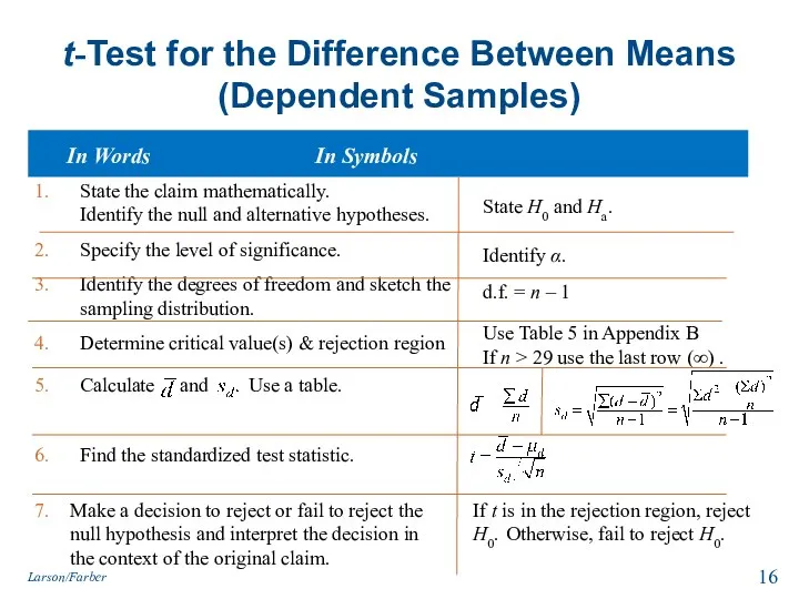
t-Test for the Difference Between Means (Dependent Samples)
State the claim mathematically.
t-Test for the Difference Between Means (Dependent Samples)
State the claim mathematically.
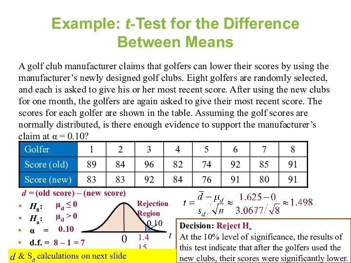
Example: t-Test for the Difference Between Means
A golf club manufacturer claims
Example: t-Test for the Difference Between Means
A golf club manufacturer claims
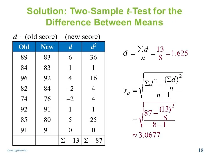
Solution: Two-Sample t-Test for the Difference Between Means
d = (old score)
Solution: Two-Sample t-Test for the Difference Between Means
d = (old score)
8.4 Two-Sample z-Test for Proportions
Used to test the difference between two
8.4 Two-Sample z-Test for Proportions
Used to test the difference between two
Two-Sample z-Test for the Difference Between Proportions
State the claim. Identify the
Two-Sample z-Test for the Difference Between Proportions
State the claim. Identify the
Example1: Two-Sample z-Test for the Difference Between Proportions
In a study of
Example1: Two-Sample z-Test for the Difference Between Proportions
In a study of
 Конспект урока и презентация по математике в 4 классе
 Тоғызқұмалақ және математика
 математика. устный счет
 Округление натуральных чисел
 Решение алгебраических и трансцендентных уравнений
 Решение задач по планиметрии
 Классификация треугольников по углам
 Свойства правильных многогранников и их применение
 Алгебра логики
 Урок математики
 Ділення з остачею
 Задачи на деление.
 Дециметр (дм)
 Нахождение дроби от числа
 Урок повторения курса геометрии 7-9
 Свойства действий над числами
 Тест по математике Решение логических задач. 5 класс
 Преподавание алгебры в 7 классе с углубленным изучением математики
 Презентация к уроку математики по программе Перспективная начальная школа
 Билеты по геометрии. Переводной экзамен. 8 класс
 Масса предметов. Килограмм
 Урок математики с презентацией в 1 классе на тему:Закрепление изученного. Проверка знаний
 Среднее арифметическое. Среднее значение величины
 Умножение положительных и отрицательных чисел
 Готовимся к ЕГЭ
 Фрагмент урока. Контрольный тест Числа больше 1000
 Аналіз характеристик КС на основі теорії марківських процесів. (Тема 5)
 Урок математики