- Evolution strategies. Chapter 4

Содержание
- 2. ES quick overview Developed: Germany in the 1970’s Early names: I. Rechenberg, H.-P. Schwefel Typically applied
- 3. ES technical summary tableau
- 4. Introductory example Task: minimimise f : Rn ? R Algorithm: “two-membered ES” using Vectors from Rn
- 5. Introductory example: pseudocde Set t = 0 Create initial point xt = 〈 x1t,…,xnt 〉 REPEAT
- 6. Introductory example: mutation mechanism z values drawn from normal distribution N(ξ,σ) mean ξ is set to
- 7. Illustration of normal distribution
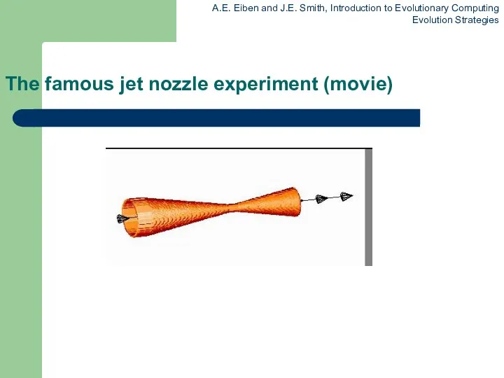
- 8. Another historical example: the jet nozzle experiment Task: to optimize the shape of a jet nozzle
- 9. Another historical example: the jet nozzle experiment cont’d Jet nozzle: the movie
- 10. The famous jet nozzle experiment (movie)
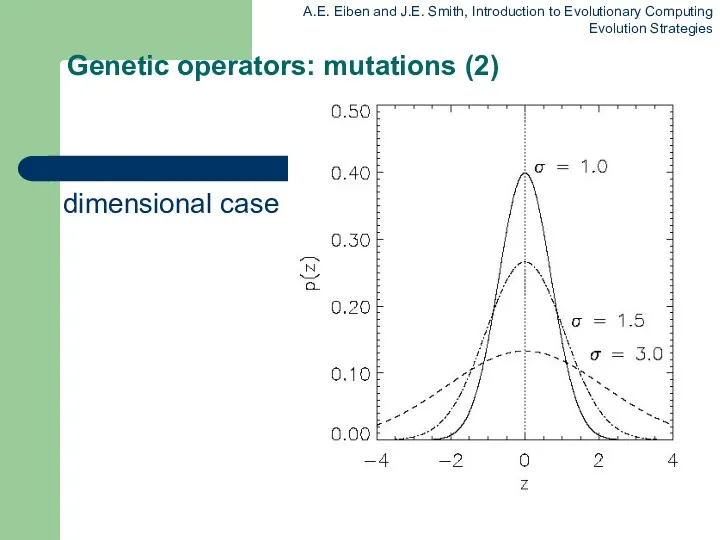
- 11. Genetic operators: mutations (2) The one dimensional case
- 12. Representation Chromosomes consist of three parts: Object variables: x1,…,xn Strategy parameters: Mutation step sizes: σ1,…,σnσ Rotation
- 13. Mutation Main mechanism: changing value by adding random noise drawn from normal distribution x’i = xi
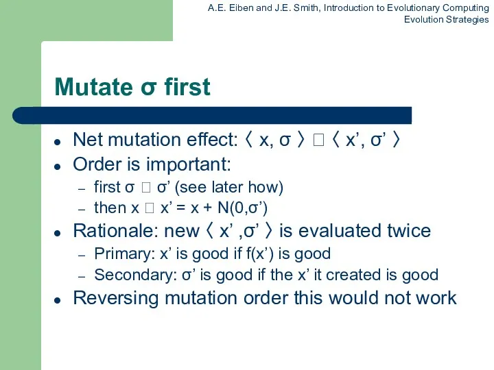
- 14. Mutate σ first Net mutation effect: 〈 x, σ 〉 ? 〈 x’, σ’ 〉 Order
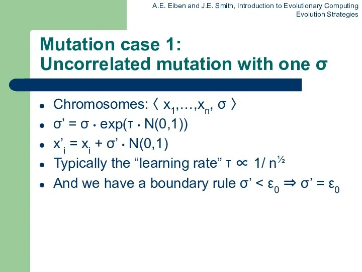
- 15. Mutation case 1: Uncorrelated mutation with one σ Chromosomes: 〈 x1,…,xn, σ 〉 σ’ = σ
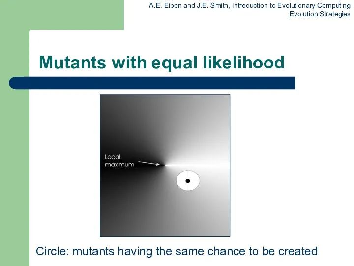
- 16. Mutants with equal likelihood Circle: mutants having the same chance to be created
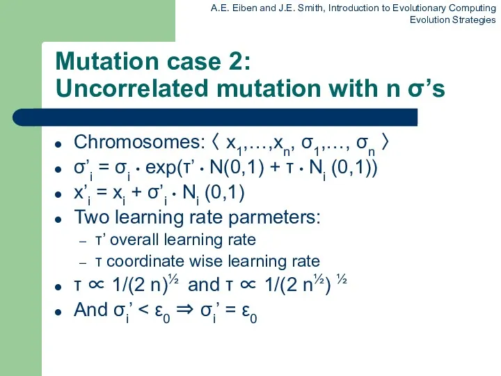
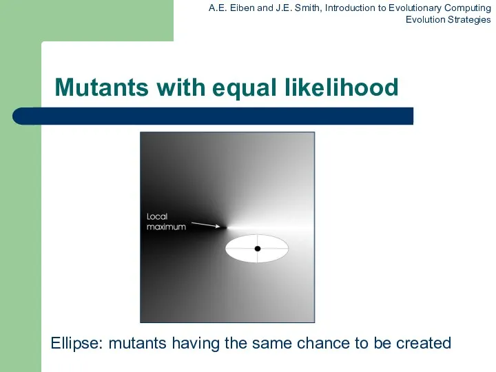
- 17. Mutation case 2: Uncorrelated mutation with n σ’s Chromosomes: 〈 x1,…,xn, σ1,…, σn 〉 σ’i =
- 18. Mutants with equal likelihood Ellipse: mutants having the same chance to be created
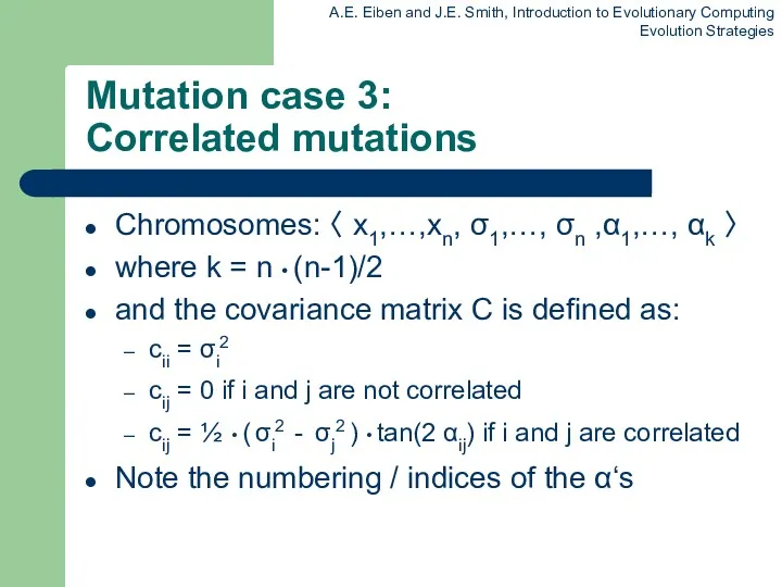
- 19. Mutation case 3: Correlated mutations Chromosomes: 〈 x1,…,xn, σ1,…, σn ,α1,…, αk 〉 where k =
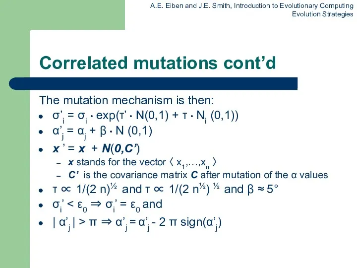
- 20. Correlated mutations cont’d The mutation mechanism is then: σ’i = σi • exp(τ’ • N(0,1) +
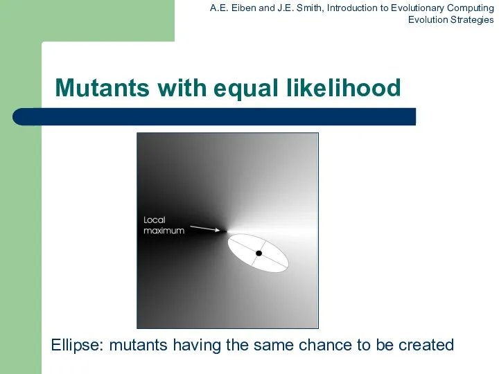
- 21. Mutants with equal likelihood Ellipse: mutants having the same chance to be created
- 22. Recombination Creates one child Acts per variable / position by either Averaging parental values, or Selecting
- 23. Names of recombinations
- 24. Parent selection Parents are selected by uniform random distribution whenever an operator needs one/some Thus: ES
- 25. Survivor selection Applied after creating λ children from the μ parents by mutation and recombination Deterministically
- 26. Survivor selection cont’d (μ+λ)-selection is an elitist strategy (μ,λ)-selection can “forget” Often (μ,λ)-selection is preferred for:
- 27. Self-adaptation illustrated Given a dynamically changing fitness landscape (optimum location shifted every 200 generations) Self-adaptive ES
- 28. Self-adaptation illustrated cont’d Changes in the fitness values (left) and the mutation step sizes (right)
- 29. Prerequisites for self-adaptation μ > 1 to carry different strategies λ > μ to generate offspring
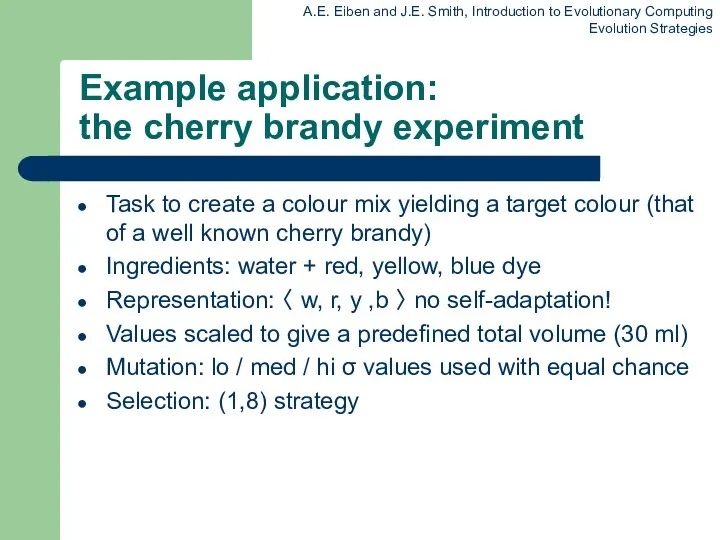
- 30. Example application: the cherry brandy experiment Task to create a colour mix yielding a target colour
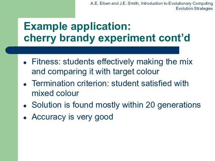
- 31. Example application: cherry brandy experiment cont’d Fitness: students effectively making the mix and comparing it with
- 33. Скачать презентацию
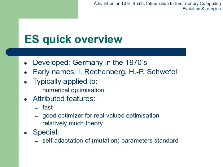
ES quick overview
Developed: Germany in the 1970’s
Early names: I. Rechenberg, H.-P.
ES quick overview
Developed: Germany in the 1970’s
Early names: I. Rechenberg, H.-P.
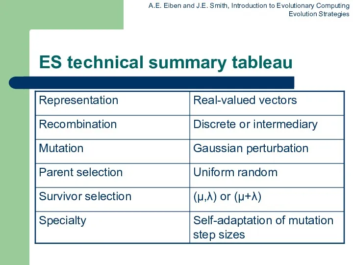
ES technical summary tableau
ES technical summary tableau
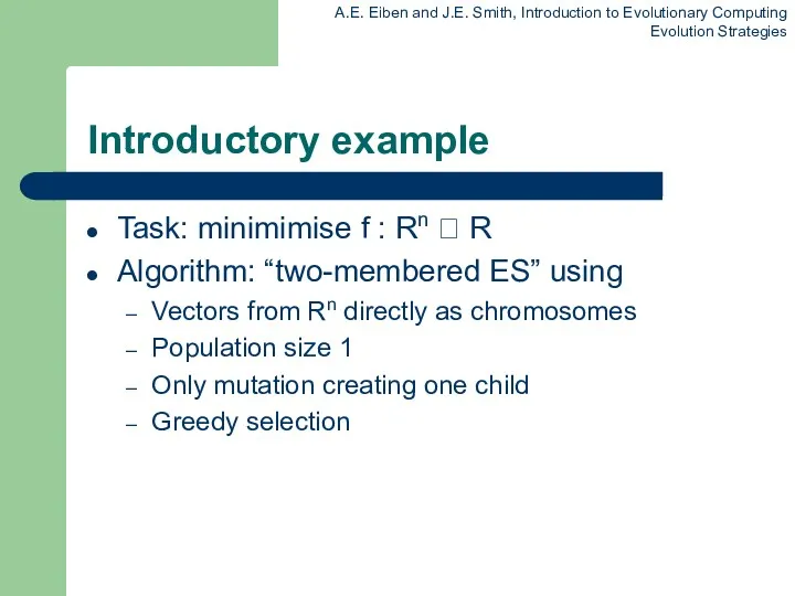
Introductory example
Task: minimimise f : Rn ? R
Algorithm: “two-membered ES” using
Introductory example
Task: minimimise f : Rn ? R
Algorithm: “two-membered ES” using
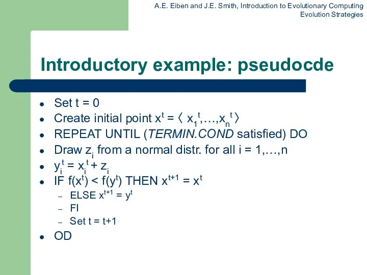
Introductory example: pseudocde
Set t = 0
Create initial point xt = 〈
Introductory example: pseudocde
Set t = 0
Create initial point xt = 〈
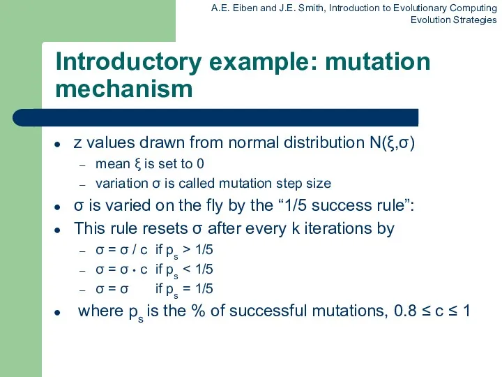
Introductory example: mutation mechanism
z values drawn from normal distribution N(ξ,σ)
mean
Introductory example: mutation mechanism
z values drawn from normal distribution N(ξ,σ)
mean
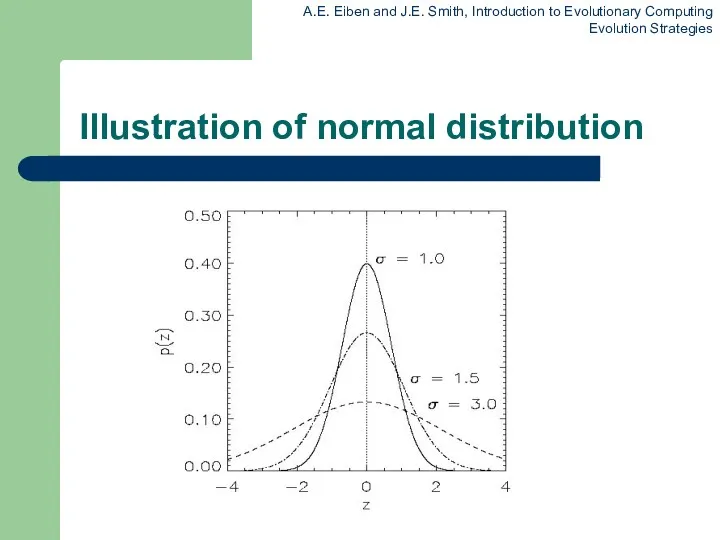
Illustration of normal distribution
Illustration of normal distribution
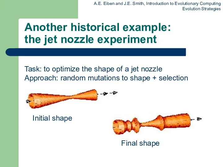
Another historical example:
the jet nozzle experiment
Task: to optimize the shape of
Another historical example:
the jet nozzle experiment
Task: to optimize the shape of
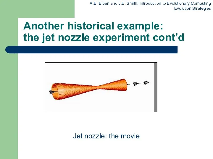
Another historical example:
the jet nozzle experiment cont’d
Jet nozzle: the movie
Another historical example:
the jet nozzle experiment cont’d
Jet nozzle: the movie
The famous jet nozzle experiment (movie)
The famous jet nozzle experiment (movie)
Genetic operators: mutations (2)
The one dimensional case
Genetic operators: mutations (2)
The one dimensional case
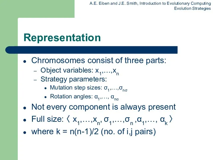
Representation
Chromosomes consist of three parts:
Object variables: x1,…,xn
Strategy parameters:
Mutation step sizes: σ1,…,σnσ
Rotation
Representation
Chromosomes consist of three parts:
Object variables: x1,…,xn
Strategy parameters:
Mutation step sizes: σ1,…,σnσ
Rotation
Mutation
Main mechanism: changing value by adding random noise drawn from normal
Mutation
Main mechanism: changing value by adding random noise drawn from normal
Mutate σ first
Net mutation effect: 〈 x, σ 〉 ? 〈
Mutate σ first
Net mutation effect: 〈 x, σ 〉 ? 〈
Mutation case 1:
Uncorrelated mutation with one σ
Chromosomes: 〈 x1,…,xn, σ 〉
Mutation case 1:
Uncorrelated mutation with one σ
Chromosomes: 〈 x1,…,xn, σ 〉
Mutants with equal likelihood
Circle: mutants having the same chance to be
Mutants with equal likelihood
Circle: mutants having the same chance to be
Mutation case 2:
Uncorrelated mutation with n σ’s
Chromosomes: 〈 x1,…,xn, σ1,…, σn
Mutation case 2:
Uncorrelated mutation with n σ’s
Chromosomes: 〈 x1,…,xn, σ1,…, σn
Mutants with equal likelihood
Ellipse: mutants having the same chance to be
Mutants with equal likelihood
Ellipse: mutants having the same chance to be
Mutation case 3:
Correlated mutations
Chromosomes: 〈 x1,…,xn, σ1,…, σn ,α1,…, αk
Mutation case 3:
Correlated mutations
Chromosomes: 〈 x1,…,xn, σ1,…, σn ,α1,…, αk
Correlated mutations cont’d
The mutation mechanism is then:
σ’i = σi • exp(τ’
Correlated mutations cont’d
The mutation mechanism is then:
σ’i = σi • exp(τ’
Mutants with equal likelihood
Ellipse: mutants having the same chance to be
Mutants with equal likelihood
Ellipse: mutants having the same chance to be
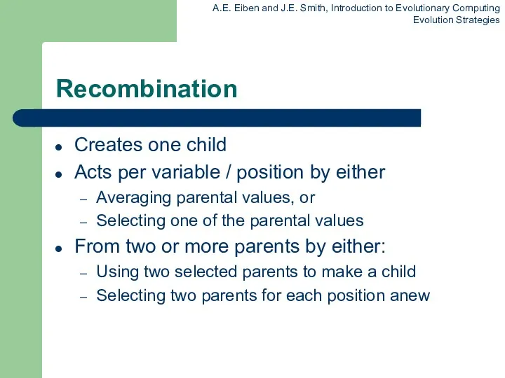
Recombination
Creates one child
Acts per variable / position by either
Averaging parental values,
Recombination
Creates one child
Acts per variable / position by either
Averaging parental values,
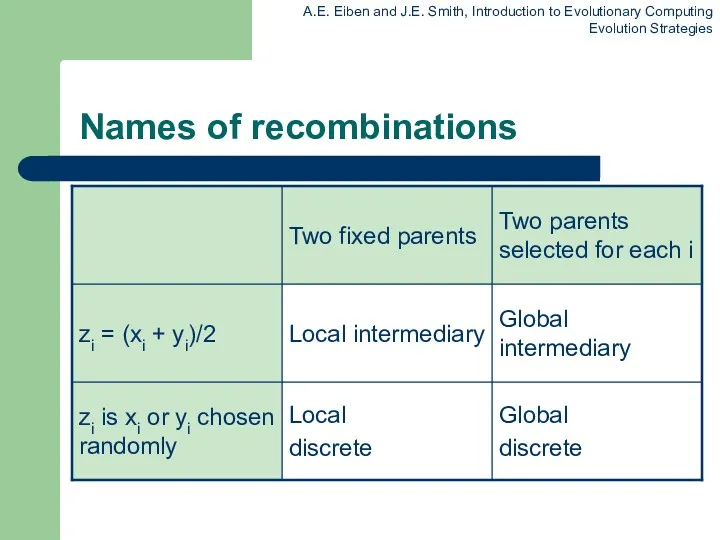
Names of recombinations
Names of recombinations
Parent selection
Parents are selected by uniform random distribution whenever an operator
Parent selection
Parents are selected by uniform random distribution whenever an operator
Survivor selection
Applied after creating λ children from the μ parents by
Survivor selection
Applied after creating λ children from the μ parents by
Survivor selection cont’d
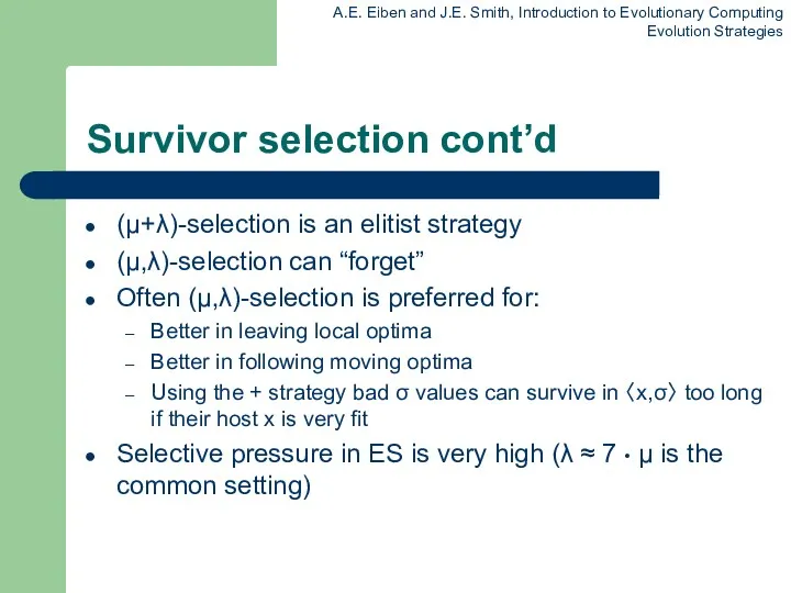
(μ+λ)-selection is an elitist strategy
(μ,λ)-selection can “forget”
Often (μ,λ)-selection is
Survivor selection cont’d
(μ+λ)-selection is an elitist strategy
(μ,λ)-selection can “forget”
Often (μ,λ)-selection is
Self-adaptation illustrated
Given a dynamically changing fitness landscape (optimum location shifted every
Self-adaptation illustrated
Given a dynamically changing fitness landscape (optimum location shifted every
Self-adaptation illustrated cont’d
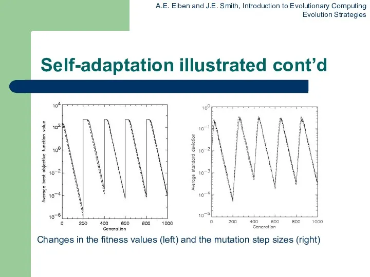
Changes in the fitness values (left) and the mutation
Self-adaptation illustrated cont’d
Changes in the fitness values (left) and the mutation
Prerequisites for self-adaptation
μ > 1 to carry different strategies
λ >
Prerequisites for self-adaptation
μ > 1 to carry different strategies
λ >
Example application:
the cherry brandy experiment
Task to create a colour mix
Example application:
the cherry brandy experiment
Task to create a colour mix
Example application:
cherry brandy experiment cont’d
Fitness: students effectively making the mix
Example application:
cherry brandy experiment cont’d
Fitness: students effectively making the mix
 Презентация Разные способы решения квадратных уравнений
 Математизация научных исследований в исторической науке
 Сложение и вычитание в пределах 100
 Своя игра. Внеклассное мероприятие по математике в 4 классе
 Презентация Урок - турнир по математике в пределах 1000 работа в группах
 Презентация для учащихся 2 класса по математике (автор Л.Г. Петерсон) Такая загадочная Индия
 Окружность. Математика 10 класс
 Правильные многогранники. Решение задач
 Табличные случаи сложения и вычитания в пределах 10 Презентация к уроку математики 1 класс
 Основы комбинаторного анализа. Формулы простого перечисления. (Лекции 16-18)
 Линейная алгебра и аналитическая геометрия
 Треугольники. Подготовка к ОГЭ. Задание 16
 Оптимизация показателей эффективности функционирования полумарковских систем массового обслуживания в торговой организации
 Натуральный и десятичный логарифмы
 Сложение вида +7
 Сложение и вычитание вида + - 3 (закрепление).
 Презентация к уроку обучения грамоте по программе Гармония по теме Звуки речи. Повторение
 класс 11.02.22 решение дробных рациональных уравнений
 Координатная прямая и виды промежутков на ней
 Вектор. Определение. Длина (модуль) вектора
 Презентация к методической разработке Формирование представлений о времени у детей дошкольного возраста. Игра Ракета времени
 Решение задач с помощью квадратных уравнений
 12 апреля в истории Кубани. Все действия с десятичными дробями. 5 класс
 Выявление ключевых задач и ключевых проблем. Теория решения изобретательских задач
 Урок математики 3 класс Виды треугольников М.И. Моро
 Конспект урока математики Миллиметр и сантиметр 3 класс УМК Перспективная начальная школа, А.Л. Чекин
 презентация по математике Решение задач в 2 действия
 Среднее арифметическое