- Introduction to Statistics

Содержание
- 2. „There are three kinds of lies: lies, damned lies, and statistics.“ (B.Disraeli) Introduction to Statistics
- 3. Without statistics we couldn't plan our budgets, pay our taxes, enjoy games... Let's take a look
- 4. Why study statistics? Data are everywhere Statistical techniques are used to make many decisions that affect
- 5. Applications of statistical concepts in the business world Finance – correlation and regression, index numbers, time
- 6. Statistics The science of collecting, organizing, presenting, analyzing, and interpreting data to assist in making more
- 7. Types of statistics Descriptive statistics – Methods of organizing, summarizing, and presenting data in an informative
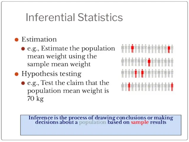
- 9. Inferential Statistics Estimation e.g., Estimate the population mean weight using the sample mean weight Hypothesis testing
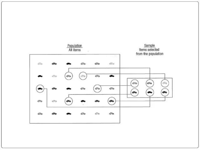
- 10. Sampling a sample should have the same characteristics as the population it is representing. Sampling can
- 11. Sampling methods Sampling methods can be: random (each member of the population has an equal chance
- 12. Random sampling methods simple random sample (each sample of the same size has an equal chance
- 13. Descriptive Statistics Collect data e.g., Survey Present data e.g., Tables and graphs Summarize data e.g., Sample
- 14. Statistical data The collection of data that are relevant to the problem being studied is commonly
- 15. Data Statistical data are usually obtained by counting or measuring items. Most data can be put
- 16. Qualitative data Qualitative data are generally described by words or letters. They are not as widely
- 17. Quantitative data Quantitative data are always numbers and are the result of counting or measuring attributes
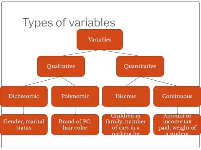
- 18. Types of variables Variables Quantitative Qualitative Dichotomic Polynomic Discrete Continuous Gender, marital status Brand of PC,
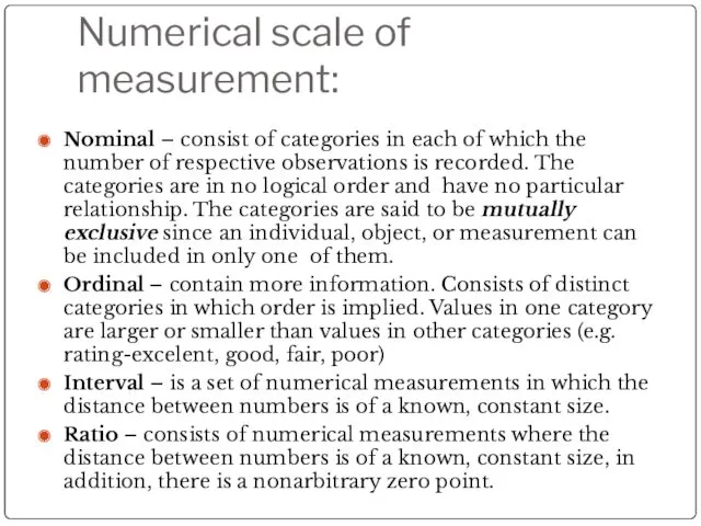
- 19. Numerical scale of measurement: Nominal – consist of categories in each of which the number of
- 20. Qualitative or Quantitative? Preferred restaurant Dollar amount of a loan Height Number of universities in Poland
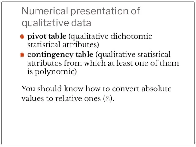
- 21. Numerical presentation of qualitative data pivot table (qualitative dichotomic statistical attributes) contingency table (qualitative statistical attributes
- 22. Frequency distributions – numerical presentation of quantitative data Frequency distribution – shows the frequency, or number
- 23. Steps for constructing a frequency distribution Determine the number of classes Determine the size of each
- 24. Frequency table absolute frequency “ni” (Data Tab?Data Analysis?Histogram) relative frequency “fi” Cumulative frequency distribution shows the
- 25. Charts and graphs Frequency distributions are good ways to present the essential aspects of data collections
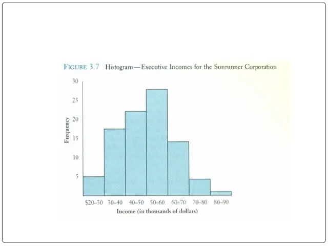
- 26. Histogram Frequently used to graphically present interval and ratio data Is often used for interval and
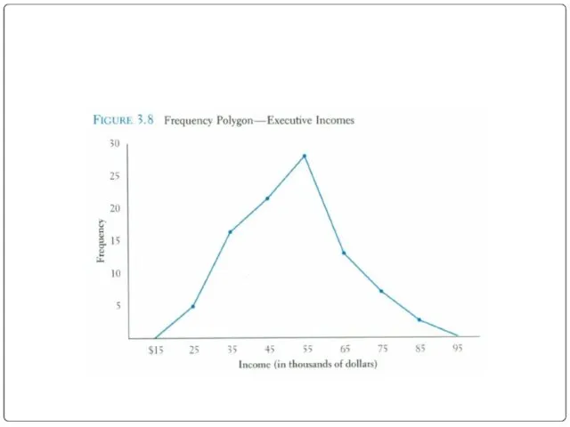
- 28. Frequency polygon Another common method for graphically presenting interval and ratio data To construct a frequency
- 30. Ogive A graph of a cumulative frequency distribution Ogive is used when one wants to determine
- 32. Pie Chart The pie chart is an effective way of displaying the percentage breakdown of data
- 33. Pie Chart
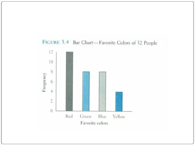
- 34. Bar chart Another common method for graphically presenting nominal and ordinal scaled data One bar is
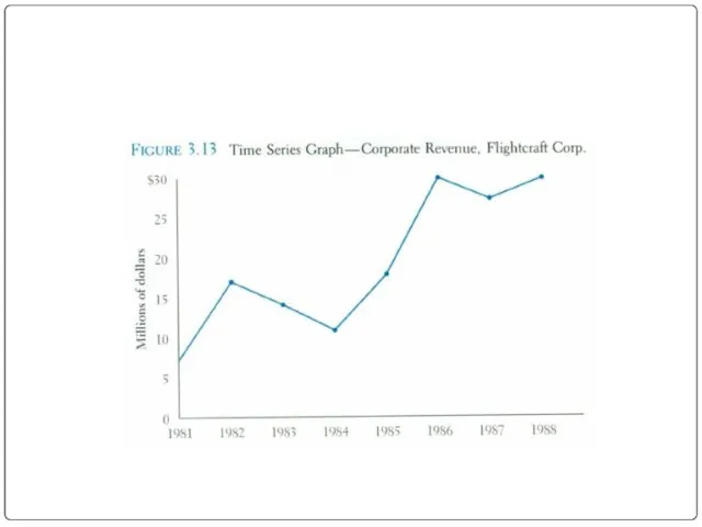
- 36. Time Series Graph The time series graph is a graph of data that have been measured
- 40. Скачать презентацию
„There are three kinds of lies: lies, damned lies, and statistics.“
„There are three kinds of lies: lies, damned lies, and statistics.“
Without statistics we couldn't plan our budgets, pay our taxes, enjoy
Without statistics we couldn't plan our budgets, pay our taxes, enjoy
Why study statistics?
Data are everywhere
Statistical techniques are used to make many
Why study statistics?
Data are everywhere
Statistical techniques are used to make many
Applications of statistical concepts in the business world
Finance – correlation and
Applications of statistical concepts in the business world
Finance – correlation and
Statistics
The science of collecting, organizing, presenting, analyzing, and interpreting data to
Statistics
The science of collecting, organizing, presenting, analyzing, and interpreting data to
Types of statistics
Descriptive statistics – Methods of organizing, summarizing, and presenting
Types of statistics
Descriptive statistics – Methods of organizing, summarizing, and presenting
Inferential Statistics
Estimation
e.g., Estimate the population mean weight using the sample mean
Inferential Statistics
Estimation
e.g., Estimate the population mean weight using the sample mean
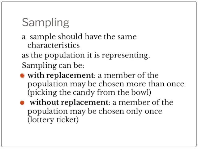
Sampling
a sample should have the same characteristics
as the population it is
Sampling
a sample should have the same characteristics
as the population it is
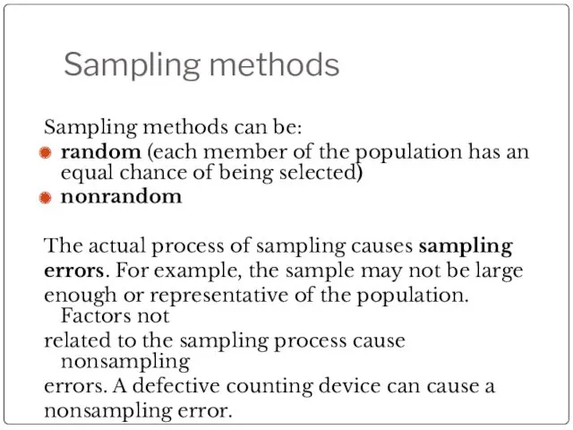
Sampling methods
Sampling methods can be:
random (each member of the population has
Sampling methods
Sampling methods can be:
random (each member of the population has
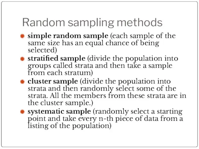
Random sampling methods
simple random sample (each sample of the same size
Random sampling methods
simple random sample (each sample of the same size
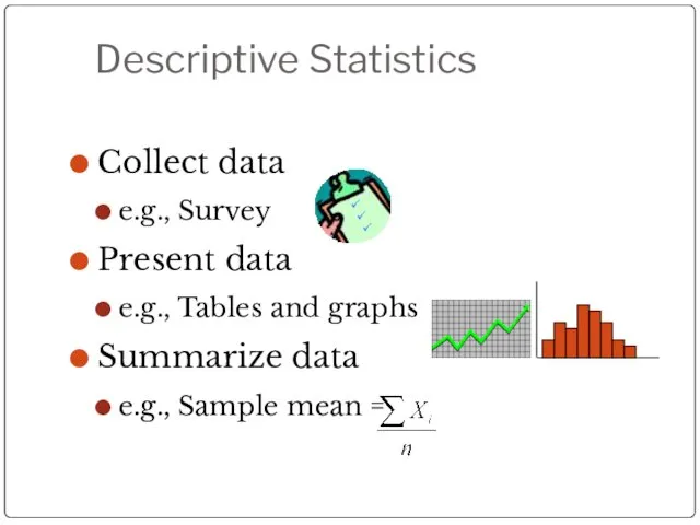
Descriptive Statistics
Collect data
e.g., Survey
Present data
e.g., Tables and graphs
Summarize data
e.g., Sample mean
Descriptive Statistics
Collect data
e.g., Survey
Present data
e.g., Tables and graphs
Summarize data
e.g., Sample mean
Statistical data
The collection of data that are relevant to the problem
Statistical data
The collection of data that are relevant to the problem
Data
Statistical data are usually obtained by counting or measuring items. Most
Data
Statistical data are usually obtained by counting or measuring items. Most
Qualitative data
Qualitative data are generally described by words or
letters. They are
Qualitative data
Qualitative data are generally described by words or
letters. They are
Quantitative data
Quantitative data are always numbers and are the
result of counting
Quantitative data
Quantitative data are always numbers and are the
result of counting
Types of variables
Variables
Quantitative
Qualitative
Dichotomic
Polynomic
Discrete
Continuous
Gender, marital status
Brand of PC, hair color
Children in family,
Types of variables
Variables
Quantitative
Qualitative
Dichotomic
Polynomic
Discrete
Continuous
Gender, marital status
Brand of PC, hair color
Children in family,
Numerical scale of measurement:
Nominal – consist of categories in each of
Numerical scale of measurement:
Nominal – consist of categories in each of
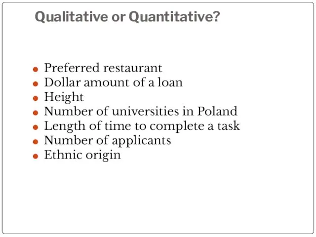
Qualitative or Quantitative?
Preferred restaurant
Dollar amount of a loan
Height
Number of universities
Qualitative or Quantitative?
Preferred restaurant
Dollar amount of a loan
Height
Number of universities
Numerical presentation of qualitative data
pivot table (qualitative dichotomic statistical attributes)
contingency table
Numerical presentation of qualitative data
pivot table (qualitative dichotomic statistical attributes)
contingency table

Frequency distributions – numerical presentation of quantitative data
Frequency distribution – shows
Frequency distributions – numerical presentation of quantitative data
Frequency distribution – shows
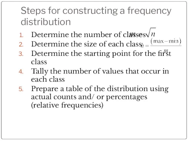
Steps for constructing a frequency distribution
Determine the number of classes
Determine the
Steps for constructing a frequency distribution
Determine the number of classes
Determine the
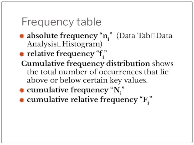
Frequency table
absolute frequency “ni” (Data Tab?Data Analysis?Histogram)
relative frequency “fi”
Cumulative frequency
Frequency table
absolute frequency “ni” (Data Tab?Data Analysis?Histogram)
relative frequency “fi”
Cumulative frequency
Charts and graphs
Frequency distributions are good ways to present the essential
Charts and graphs
Frequency distributions are good ways to present the essential
Histogram
Frequently used to graphically present interval and ratio data
Is often used
Histogram
Frequently used to graphically present interval and ratio data
Is often used
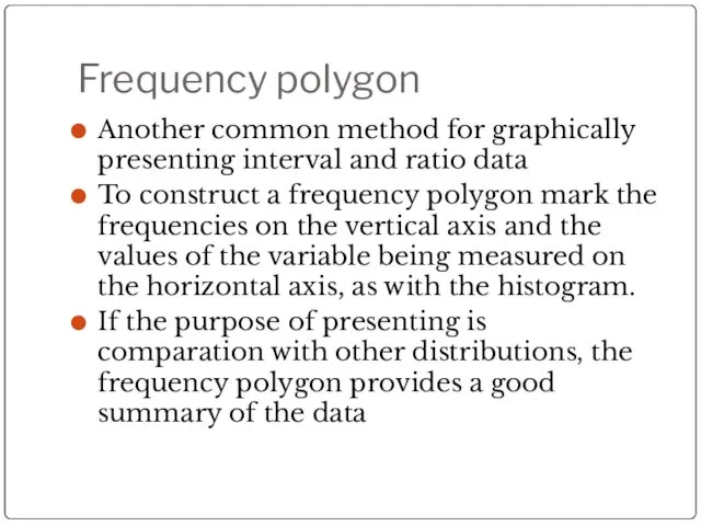
Frequency polygon
Another common method for graphically presenting interval and ratio data
To
Frequency polygon
Another common method for graphically presenting interval and ratio data
To
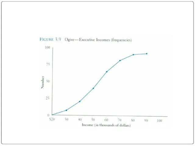
Ogive
A graph of a cumulative frequency distribution
Ogive is used when one
Ogive
A graph of a cumulative frequency distribution
Ogive is used when one
Pie Chart
The pie chart is an effective way of displaying the
Pie Chart
The pie chart is an effective way of displaying the
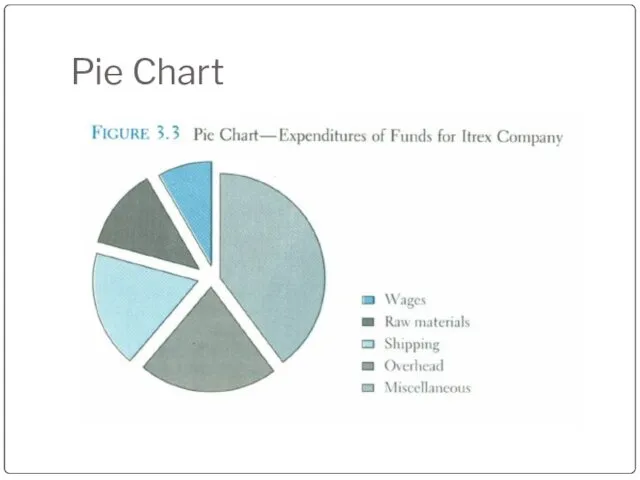
Pie Chart
Pie Chart
Bar chart
Another common method for graphically presenting nominal and ordinal scaled
Bar chart
Another common method for graphically presenting nominal and ordinal scaled
Time Series Graph
The time series graph is a graph of data
Time Series Graph
The time series graph is a graph of data

 Взаємне розміщення площини і кулі у просторі
 Благоприятствующие элементарные события. Вероятность события
 Решение систем уравнений с двумя неизвестными
 Урок математики 1класс. Точки и линии
 Теоретическая модель жизни пчелиных колоний
 Оригами как метод ознакомления детей с формой предметов.
 Презентация-игра Помогите сказке
 Математика. 1 класс. Урок 55. Числа 0-10 - Презентация
 Упрощение выражений. 5 класс
 Задачи теории вероятностей. Повторение к ГИА и ЕГЭ
 Алгоритм сложения трёхзначных чисел
 Столбчатые диаграммы. Демонстрационный материал. 6 класс
 Основы математической обработки информации
 Теорема Виета
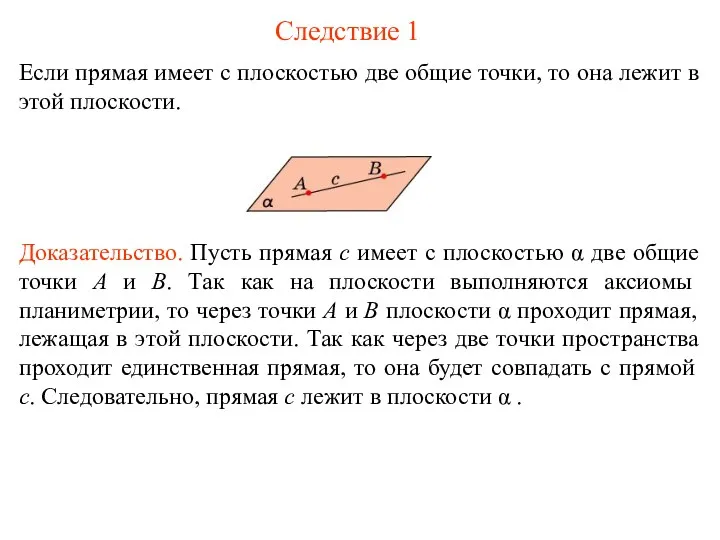 Следствие из аксиом стереометрии
 Десятичные дроби. 5 класс
 Рациональные уравнения как математические модели реальных ситуаций
 Подобие в геометрии. Подобные треугольники
 Прямоугольный параллелепипед
 Деление с остатком
 Доказательство теоремы Пифагора
 Топологические объекты
 Основы векторной алгебры. Векторы на плоскости и в пространстве
 Целеполагание как этап современного урока в условиях ФГОС
 Урок математики 1 класс Тема: Число восемь. Цифра 8.
 ОГЭ Модуль Реальная математика
 Геометрична фігура трикутник. (7 класс)
 Конспект урока математики 2 класс по системе Занкова (И.И.Аргинская) Тема урока: Умножение