- The Normal and other Continuous Distributions

Содержание
- 2. 7.1 The Standard Deviation as a Ruler Recall that z-scores provide a standard way to compare
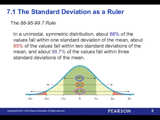
- 3. 7.1 The Standard Deviation as a Ruler The 68-95-99.7 Rule In a unimodal, symmetric distribution, about
- 4. 7.1 The Standard Deviation as a Ruler For Example: On August 8, 2011, the Dow dropped
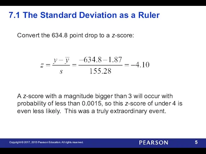
- 5. 7.1 The Standard Deviation as a Ruler Convert the 634.8 point drop to a z-score: A
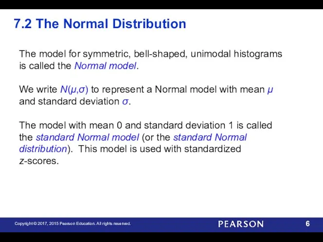
- 6. 7.2 The Normal Distribution The model for symmetric, bell-shaped, unimodal histograms is called the Normal model.
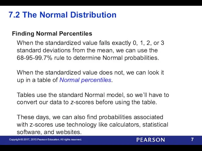
- 7. 7.2 The Normal Distribution Finding Normal Percentiles When the standardized value falls exactly 0, 1, 2,
- 8. 7.2 The Normal Distribution Example 1: Each Scholastic Aptitude Test (SAT) has a distribution that is
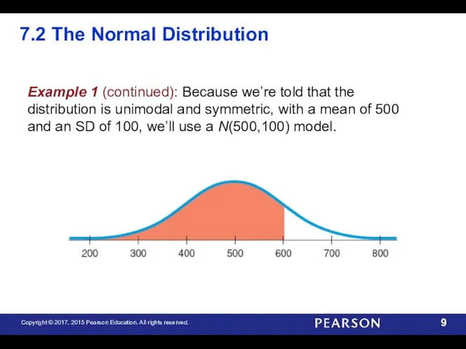
- 9. 7.2 The Normal Distribution Example 1 (continued): Because we’re told that the distribution is unimodal and
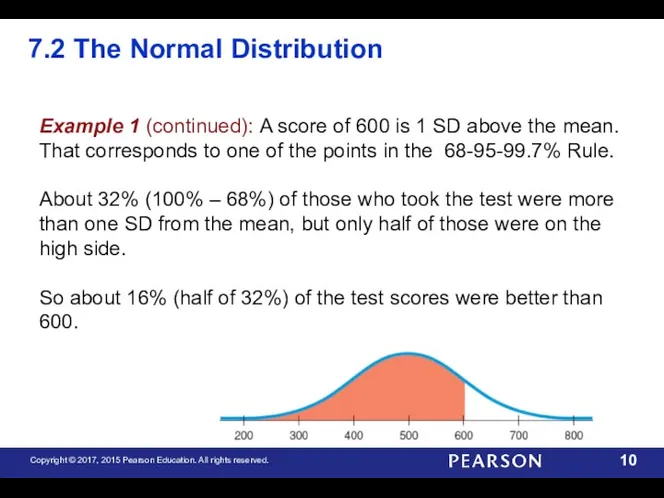
- 10. 7.2 The Normal Distribution Example 1 (continued): A score of 600 is 1 SD above the
- 11. 7.2 The Normal Distribution Example 2: Assuming the SAT scores are nearly normal with N(500,100), what
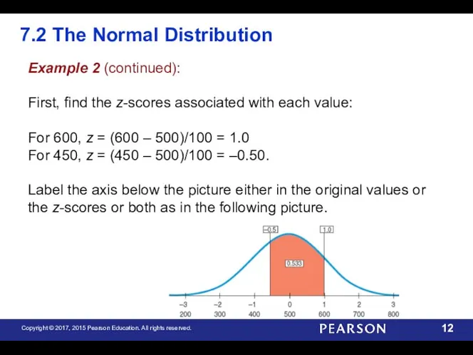
- 12. 7.2 The Normal Distribution Example 2 (continued): First, find the z-scores associated with each value: For
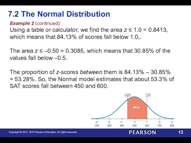
- 13. 7.2 The Normal Distribution Example 2 (continued): Using a table or calculator, we find the area
- 14. 7.2 The Normal Distribution Sometimes we start with areas and are asked to work backward to
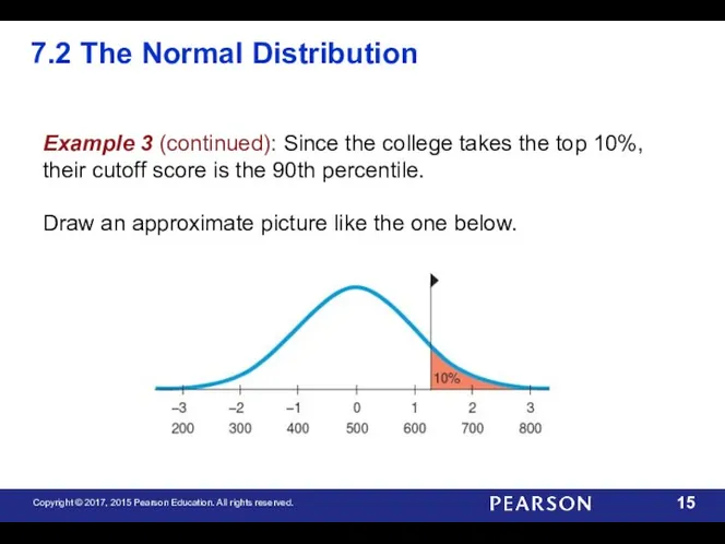
- 15. 7.2 The Normal Distribution Example 3 (continued): Since the college takes the top 10%, their cutoff
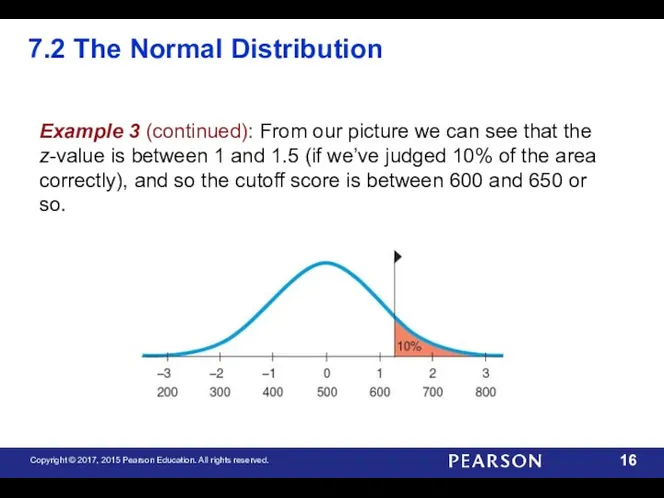
- 16. 7.2 The Normal Distribution Example 3 (continued): From our picture we can see that the z-value
- 17. 7.2 The Normal Distribution Example 3 (continued): Using technology, you will be able to select the
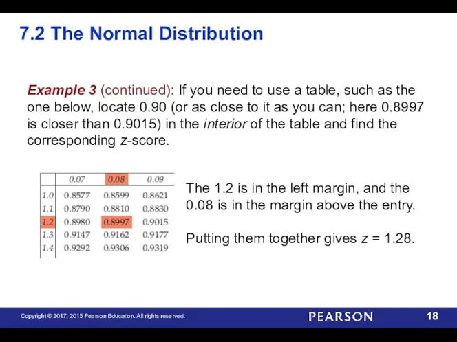
- 18. 7.2 The Normal Distribution Example 3 (continued): If you need to use a table, such as
- 19. 7.2 The Normal Distribution Example 3 (continued): Convert the z-score back to the original units. A
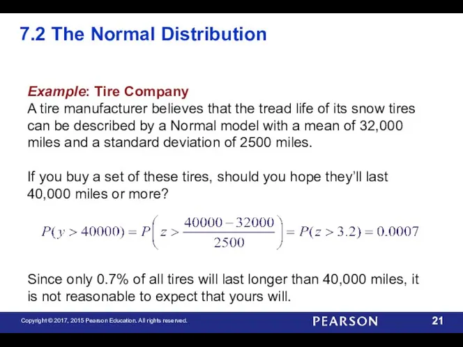
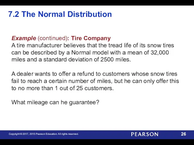
- 20. 7.2 The Normal Distribution Example: Tire Company A tire manufacturer believes that the tread life of
- 21. 7.2 The Normal Distribution Example: Tire Company A tire manufacturer believes that the tread life of
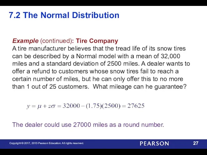
- 22. 7.2 The Normal Distribution Example (continued): Tire Company A tire manufacturer believes that the tread life
- 23. 7.2 The Normal Distribution Example (continued): Tire Company A tire manufacturer believes that the tread life
- 24. 7.2 The Normal Distribution Example (continued): Tire Company A tire manufacturer believes that the tread life
- 25. 7.2 The Normal Distribution Example (continued): Tire Company A tire manufacturer believes that the tread life
- 26. 7.2 The Normal Distribution Example (continued): Tire Company A tire manufacturer believes that the tread life
- 27. 7.2 The Normal Distribution Example (continued): Tire Company A tire manufacturer believes that the tread life
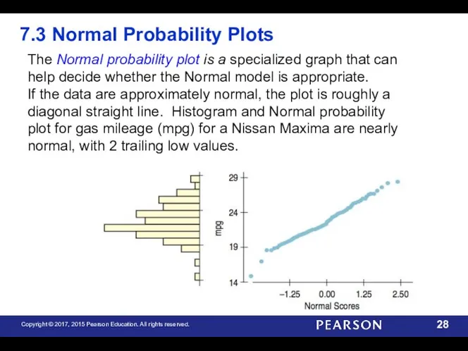
- 28. 7.3 Normal Probability Plots The Normal probability plot is a specialized graph that can help decide
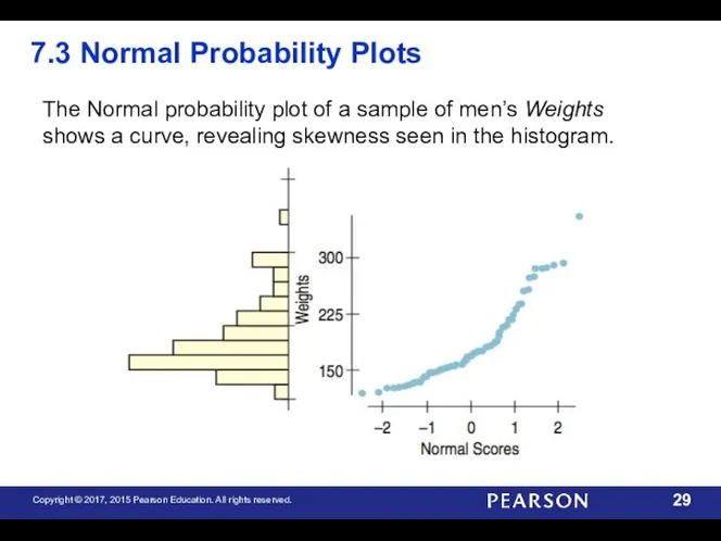
- 29. 7.3 Normal Probability Plots The Normal probability plot of a sample of men’s Weights shows a
- 30. 7.4 The Distribution of Sums of Normals Normal models have many special properties. One of these
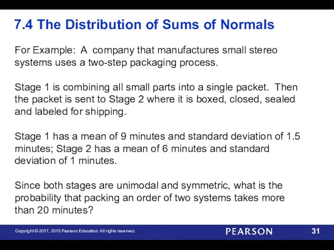
- 31. For Example: A company that manufactures small stereo systems uses a two-step packaging process. Stage 1
- 32. Normal Model Assumption - We are told both stages are unimodal and symmetric. And we know
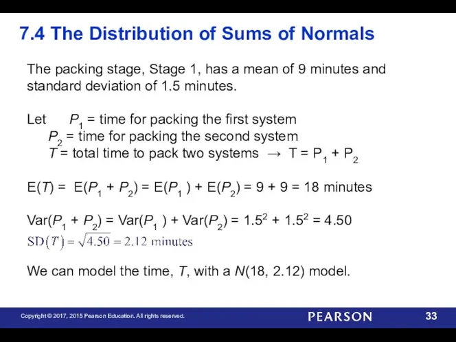
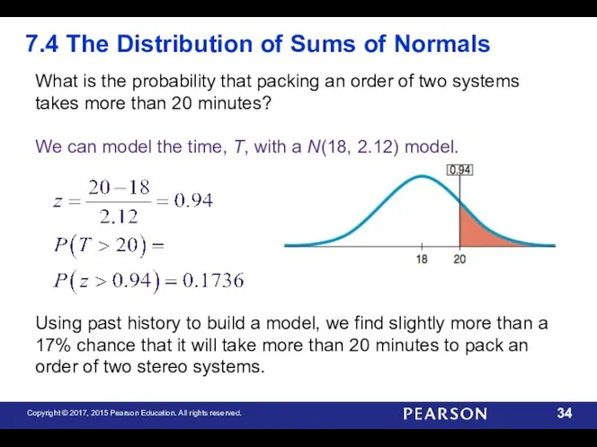
- 33. The packing stage, Stage 1, has a mean of 9 minutes and standard deviation of 1.5
- 34. What is the probability that packing an order of two systems takes more than 20 minutes?
- 35. 7.5 The Normal Approximation for the Binomial A discrete Binomial model with n trials and probability
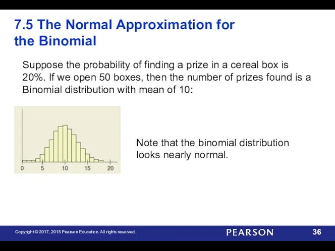
- 36. 7.5 The Normal Approximation for the Binomial Suppose the probability of finding a prize in a
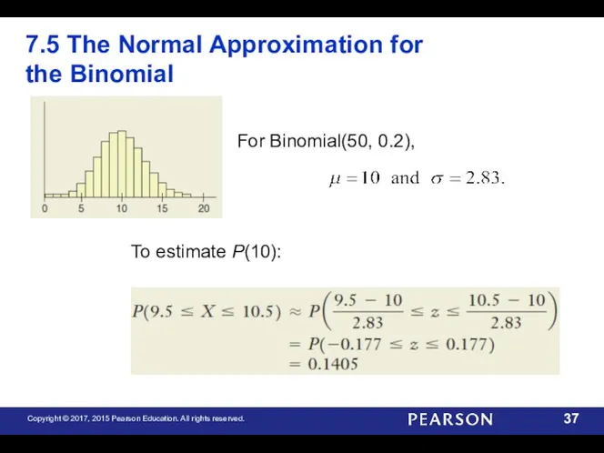
- 37. 7.5 The Normal Approximation for the Binomial For Binomial(50, 0.2), To estimate P(10):
- 38. 7.6 Other Continuous Random Variables Many phenomena in business can be modeled by continuous random variables.
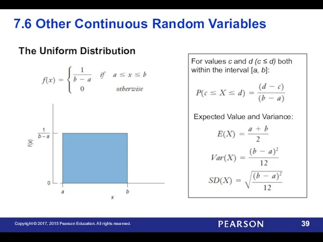
- 39. 7.6 Other Continuous Random Variables The Uniform Distribution For values c and d (c ≤ d)
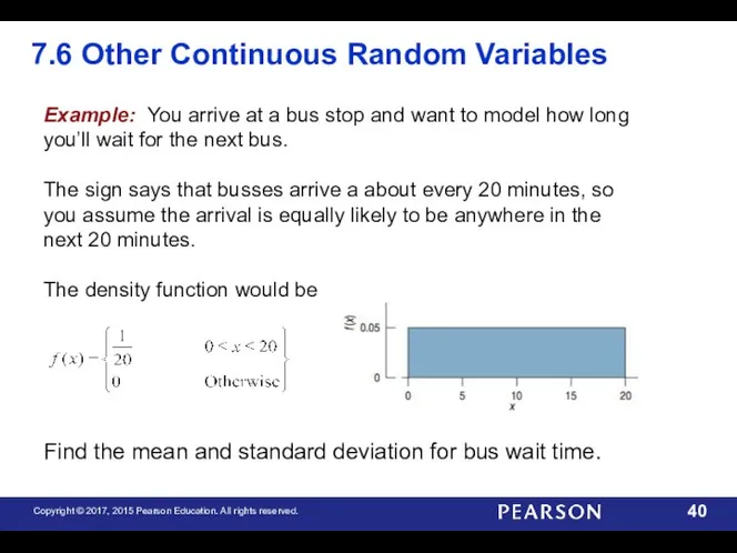
- 40. 7.6 Other Continuous Random Variables Example: You arrive at a bus stop and want to model
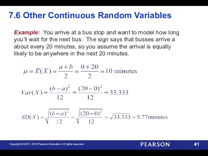
- 41. 7.6 Other Continuous Random Variables Example: You arrive at a bus stop and want to model
- 42. Probability models are still just models. Don’t assume everything’s Normal. Don’t use the Normal approximation with
- 43. What Have We Learned? Recognize normally distributed data by making a histogram and checking whether it
- 44. What Have We Learned? Understand how to use the Normal model to judge whether a value
- 46. Скачать презентацию
7.1 The Standard Deviation as a Ruler
Recall that z-scores provide a standard way
7.1 The Standard Deviation as a Ruler
Recall that z-scores provide a standard way
7.1 The Standard Deviation as a Ruler
The 68-95-99.7 Rule
In a unimodal, symmetric distribution,
7.1 The Standard Deviation as a Ruler
The 68-95-99.7 Rule
In a unimodal, symmetric distribution,
7.1 The Standard Deviation as a Ruler
For Example: On August 8, 2011, the
7.1 The Standard Deviation as a Ruler
For Example: On August 8, 2011, the
7.1 The Standard Deviation as a Ruler
Convert the 634.8 point drop to a
7.1 The Standard Deviation as a Ruler
Convert the 634.8 point drop to a
7.2 The Normal Distribution
The model for symmetric, bell-shaped, unimodal histograms is called the
7.2 The Normal Distribution
The model for symmetric, bell-shaped, unimodal histograms is called the
7.2 The Normal Distribution
Finding Normal Percentiles
When the standardized value falls exactly 0, 1,
7.2 The Normal Distribution
Finding Normal Percentiles
When the standardized value falls exactly 0, 1,
7.2 The Normal Distribution
Example 1: Each Scholastic Aptitude Test (SAT) has a distribution
7.2 The Normal Distribution
Example 1: Each Scholastic Aptitude Test (SAT) has a distribution
7.2 The Normal Distribution
Example 1 (continued): Because we’re told that the distribution is
7.2 The Normal Distribution
Example 1 (continued): Because we’re told that the distribution is
7.2 The Normal Distribution
Example 1 (continued): A score of 600 is 1 SD
7.2 The Normal Distribution
Example 1 (continued): A score of 600 is 1 SD
7.2 The Normal Distribution
Example 2: Assuming the SAT scores are nearly normal with
7.2 The Normal Distribution
Example 2: Assuming the SAT scores are nearly normal with
7.2 The Normal Distribution
Example 2 (continued):
First, find the z-scores associated with each
7.2 The Normal Distribution
Example 2 (continued):
First, find the z-scores associated with each
7.2 The Normal Distribution
Example 2 (continued):
Using a table or calculator, we find
7.2 The Normal Distribution
Example 2 (continued):
Using a table or calculator, we find
7.2 The Normal Distribution
Sometimes we start with areas and are asked to work
7.2 The Normal Distribution
Sometimes we start with areas and are asked to work
7.2 The Normal Distribution
Example 3 (continued): Since the college takes the top 10%,
7.2 The Normal Distribution
Example 3 (continued): Since the college takes the top 10%,
7.2 The Normal Distribution
Example 3 (continued): From our picture we can see that
7.2 The Normal Distribution
Example 3 (continued): From our picture we can see that
7.2 The Normal Distribution
Example 3 (continued): Using technology, you will be able to
7.2 The Normal Distribution
Example 3 (continued): Using technology, you will be able to
7.2 The Normal Distribution
Example 3 (continued): If you need to use a table,
7.2 The Normal Distribution
Example 3 (continued): If you need to use a table,
7.2 The Normal Distribution
Example 3 (continued): Convert the z-score back to the original
7.2 The Normal Distribution
Example 3 (continued): Convert the z-score back to the original
7.2 The Normal Distribution
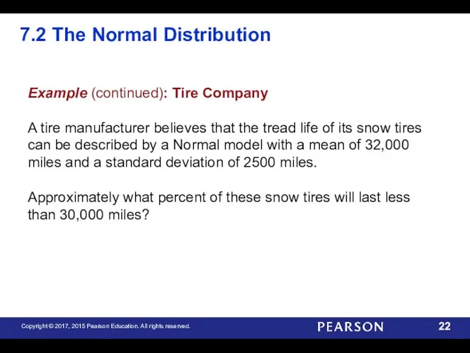
Example: Tire Company
A tire manufacturer believes that the tread life
7.2 The Normal Distribution
Example: Tire Company
A tire manufacturer believes that the tread life
7.2 The Normal Distribution
Example: Tire Company
A tire manufacturer believes that the tread life
7.2 The Normal Distribution
Example: Tire Company
A tire manufacturer believes that the tread life
7.2 The Normal Distribution
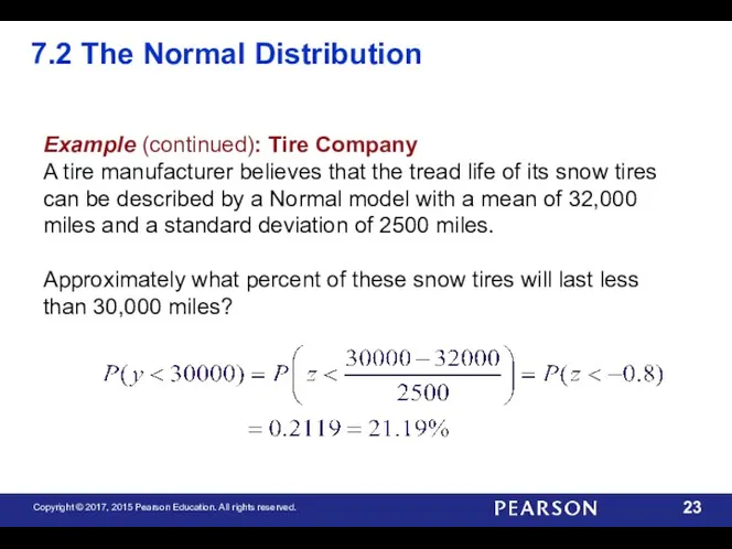
Example (continued): Tire Company
A tire manufacturer believes that the tread
7.2 The Normal Distribution
Example (continued): Tire Company
A tire manufacturer believes that the tread
7.2 The Normal Distribution
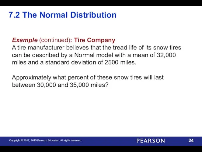
Example (continued): Tire Company
A tire manufacturer believes that the tread
7.2 The Normal Distribution
Example (continued): Tire Company
A tire manufacturer believes that the tread
7.2 The Normal Distribution
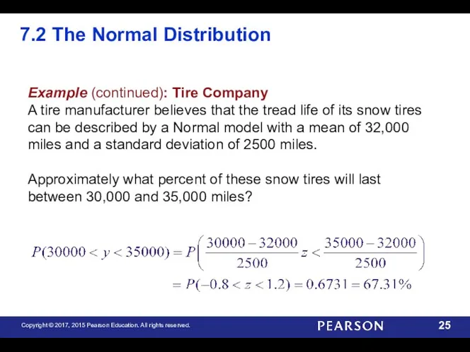
Example (continued): Tire Company
A tire manufacturer believes that the tread
7.2 The Normal Distribution
Example (continued): Tire Company
A tire manufacturer believes that the tread
7.2 The Normal Distribution
Example (continued): Tire Company
A tire manufacturer believes that the tread
7.2 The Normal Distribution
Example (continued): Tire Company
A tire manufacturer believes that the tread
7.2 The Normal Distribution
Example (continued): Tire Company
A tire manufacturer believes that the tread
7.2 The Normal Distribution
Example (continued): Tire Company
A tire manufacturer believes that the tread
7.2 The Normal Distribution
Example (continued): Tire Company
A tire manufacturer believes that the tread
7.2 The Normal Distribution
Example (continued): Tire Company
A tire manufacturer believes that the tread
7.3 Normal Probability Plots
The Normal probability plot is a specialized graph that can
7.3 Normal Probability Plots
The Normal probability plot is a specialized graph that can
7.3 Normal Probability Plots
The Normal probability plot of a sample of men’s Weights
7.3 Normal Probability Plots
The Normal probability plot of a sample of men’s Weights
7.4 The Distribution of Sums of Normals
Normal models have many special properties. One
7.4 The Distribution of Sums of Normals
Normal models have many special properties. One
For Example: A company that manufactures small stereo systems uses a two-step packaging
For Example: A company that manufactures small stereo systems uses a two-step packaging
Normal Model Assumption - We are told both stages are unimodal and symmetric.
The packing stage, Stage 1, has a mean of 9 minutes and standard
The packing stage, Stage 1, has a mean of 9 minutes and standard
What is the probability that packing an order of two systems takes more
What is the probability that packing an order of two systems takes more
7.5 The Normal Approximation for the Binomial
A discrete Binomial model with n trials
7.5 The Normal Approximation for the Binomial
A discrete Binomial model with n trials
7.5 The Normal Approximation for the Binomial
Suppose the probability of finding a prize
7.5 The Normal Approximation for the Binomial
Suppose the probability of finding a prize
7.5 The Normal Approximation for the Binomial
For Binomial(50, 0.2),
To estimate P(10):
7.5 The Normal Approximation for the Binomial
For Binomial(50, 0.2),
To estimate P(10):
7.6 Other Continuous Random Variables
Many phenomena in business can be modeled by continuous
7.6 Other Continuous Random Variables
Many phenomena in business can be modeled by continuous
7.6 Other Continuous Random Variables
The Uniform Distribution
For values c and d (c ≤
7.6 Other Continuous Random Variables
The Uniform Distribution
For values c and d (c ≤
7.6 Other Continuous Random Variables
Example: You arrive at a bus stop and want
7.6 Other Continuous Random Variables
Example: You arrive at a bus stop and want
7.6 Other Continuous Random Variables
Example: You arrive at a bus stop and want
7.6 Other Continuous Random Variables
Example: You arrive at a bus stop and want
Probability models are still just models.
Don’t assume everything’s Normal.
Don’t
Probability models are still just models.
Don’t assume everything’s Normal.
Don’t
What Have We Learned?
Recognize normally distributed data by making a histogram and checking
What Have We Learned?
Recognize normally distributed data by making a histogram and checking
What Have We Learned?
Understand how to use the Normal model to judge whether
What Have We Learned?
Understand how to use the Normal model to judge whether
 Четыре периода развития математики
 Формула площади прямоугольника
 Trigonometry 1
 Презентация и конспект урока Круглые двузначные числа Урок математики в 1 классе
 Неопределенность измерений
 Плоские фигуры - многоугольники. Объемные фигуры
 Шаблоны презентаций по математике
 Множества. Понятие множества
 Геометрии Евклида как первая научная система
 Использование матриц при решении экономических задач
 Розв'язування задач. Самостійна робота
 Угол между векторами. Скалярное произведение векторов
 Гамильтоновы и Эйлеровы графы
 Площадь трапеции
 Сфера и шар. Теорема
 In elementary algebra, the binomial
 презентация к уроку в 4 классе. Тема: Задачи на движение
 Преобразование графиков функций
 Презентация Образование чисел второго десятка
 Умножение и деление обыкновенной дроби на натуральное число. (Урок 72)
 Этапы решения математических задач
 Бином Ньютона
 Единицы длины – дециметр
 Математическая логика и теория алгоритмов
 Симметричные фигуры
 Луч и угол. 7 класс
 Функції та їх графіки
 Пирамида в задачах ЕГЭ