- System reliability

Содержание
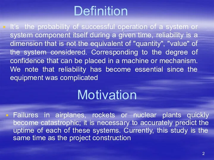
- 2. Definition It’s the probability of successful operation of a system or system component itself during a
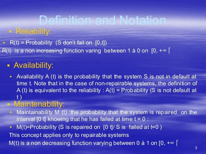
- 3. Definition and Notation Reliability: R(t) = Probability (S don’t fail on [0,t]) R(t) is a non
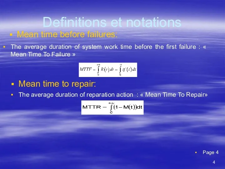
- 4. Definitions et notations Mean time before failures: Mean time to repair: Page 4 The average duration
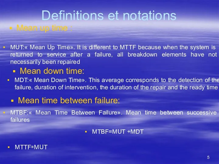
- 5. Definitions et notations Mean up time : MUT:« Mean Up Time». It is different to MTTF
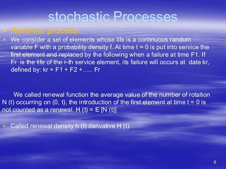
- 6. stochastic Processes Renewal process: We consider a set of elements whose life is a continuous random
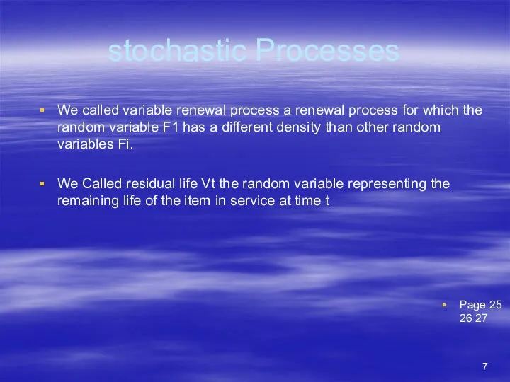
- 7. stochastic Processes We called variable renewal process a renewal process for which the random variable F1
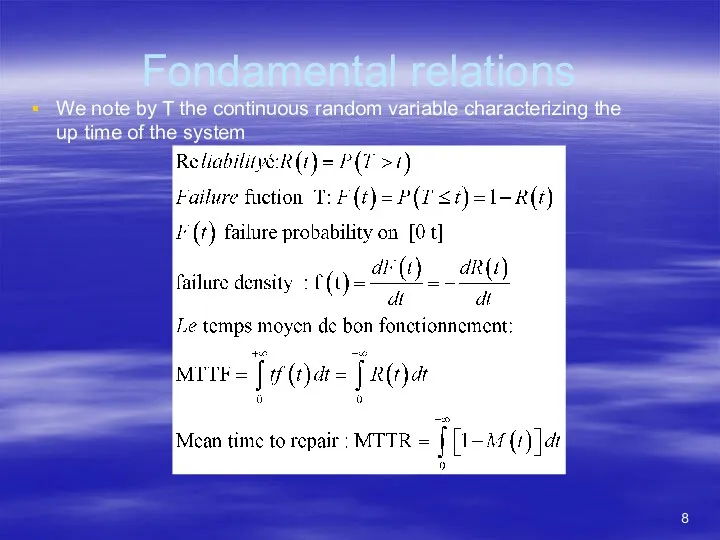
- 8. Fondamental relations We note by T the continuous random variable characterizing the up time of the
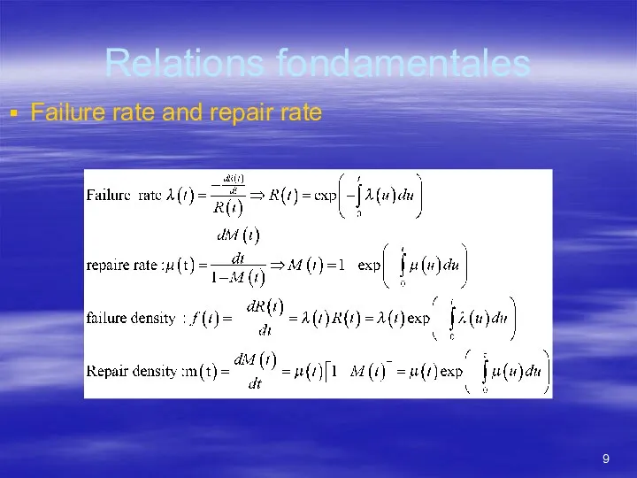
- 9. Relations fondamentales Failure rate and repair rate
- 10. Method of determination of the material failure law « New material » Experimentation The Principe consists
- 11. Method of determination of the material failure law « New material » Case 1 N≥50 :
- 12. Method of determination of the material failure law « New material » Case 1 N≥50 :
- 13. Method of determination of the material failure law « New material » Case 1 N≥50 :
- 14. Method of determination of the material failure law « New material » Case 2 N -
- 15. Method of determination of the material failure law « New material » Case 2 N For
- 16. Method of determination of the material failure law « New material » Plote Fi according to
- 17. Acceptance test for obtained law Case 1 N≥50 : KHI-Deux Test Compute E: E= ∑((ni-N*Pi)^2)/(N*Pi) And
- 18. Acceptance test for obtained law Case 2 N Compute D+ and D- D+ = max {(i/N)-F(ti))},
- 19. Principal law used in industry and research in reliability frame
- 20. Usuel discret law
- 21. It’s a constant law Dirac:
- 22. Bernoulli: Parameter is p defined by p=P(A), notation X →B(1,p) Dem FIGURE EXEMPLE page 66 67
- 23. Parameters n and p=P(A) « binomiale »: Notation X →B(n,p) Dem EXEMPLE page 69
- 24. Parameters λ>0 « Poisson » : Notation X →P(λ) Dem EXEMPLE page 72 73 74
- 25. « Pascal »: Dem page 74 75 Parameter k
- 26. Parameters n and y : « binomiale négative »: Dem page 75
- 27. Continuous law Dem page 77 78
- 28. « Loi uniforme »
- 29. Exponential law : Notation X →ε(θ) Dem page 78 79
- 30. Laplace-Gauss: .Notation X →N(m, σ ) Dem page 79 80-83 Parameters m and σ
- 31. Parameters p>0 and θ>0 « gamma » Dem page 84-85
- 32. Lois usuelles continues Gamma with p=n/2 and θ=1/2 (γ(n/2, 1/2)) « Khi-Deux »: Dem page 85
- 33. Si X = γ(p) and Y= γ(q), we deduce Z=X/Y = β11(p,q) « Beta": Second :
- 34. « Beta »: First Dem page 88
- 35. Parameters m and σ « log-normale »: Dem page 90
- 36. Parameters x0 (x≥x0>0) and α>0: « Pareto »: Dem page 91
- 37. Lois Weibull trois paramètres Densité de probabilité : Fonction de répartition :
- 38. Lois Weibull deux paramètres ( β,λ) Densité de probabilité : Fonction de répartition :
- 39. Structures Dem page 91 series
- 40. Structures Dem page 91 parallel Series-parallel Parallel-series
- 41. Complex Structures Bridge system Dem page 91 Theorem of Bays Exampl
- 42. Structures Dem page 91 series parallel Parallel-series Series-parallel
- 43. Structures Dem page 91 series parallel Parallel-series Series-parallel
- 45. Скачать презентацию
Definition
It’s the probability of successful operation of a system or system
Definition
It’s the probability of successful operation of a system or system
Definition and Notation
Reliability:
R(t) = Probability (S don’t fail on [0,t])
R(t) is
Definition and Notation
Reliability:
R(t) = Probability (S don’t fail on [0,t])
R(t) is
Definitions et notations
Mean time before failures:
Mean time to repair:
Page 4
The average
Definitions et notations
Mean time before failures:
Mean time to repair:
Page 4
The average
Definitions et notations
Mean up time :
MUT:« Mean Up Time». It is
Definitions et notations
Mean up time :
MUT:« Mean Up Time». It is
stochastic Processes
Renewal process:
We consider a set of elements whose life is
stochastic Processes
Renewal process:
We consider a set of elements whose life is
stochastic Processes
We called variable renewal process a renewal process for which
stochastic Processes
We called variable renewal process a renewal process for which
Fondamental relations
We note by T the continuous random variable characterizing the
Fondamental relations
We note by T the continuous random variable characterizing the
Relations fondamentales
Failure rate and repair rate
Relations fondamentales
Failure rate and repair rate
Method of determination of the material failure law
« New material »
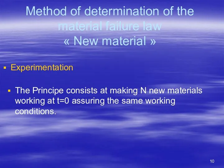
Experimentation
The Principe
Method of determination of the material failure law
« New material »
Experimentation
The Principe
Method of determination of the material failure law
« New material »
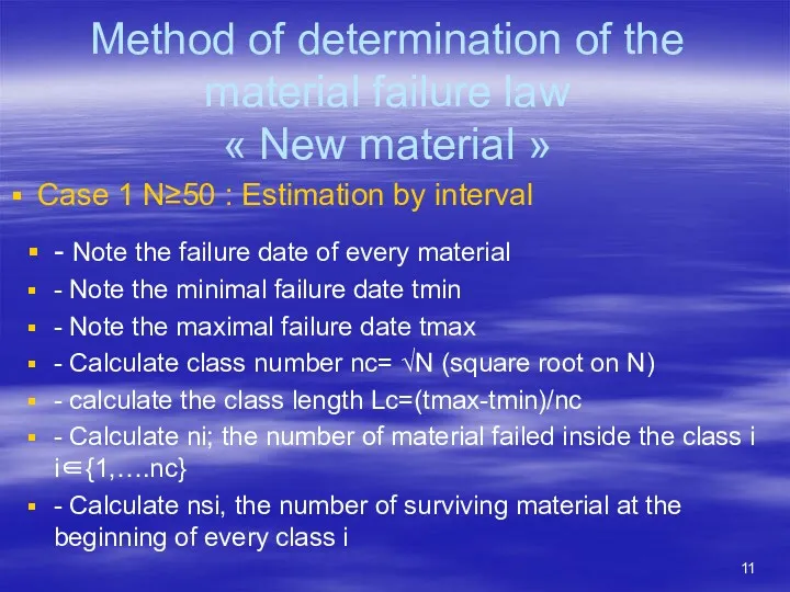
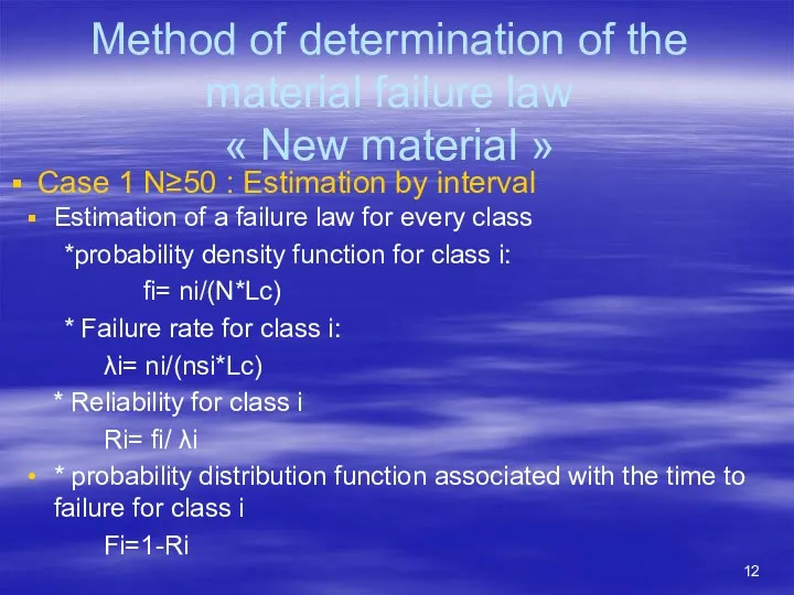
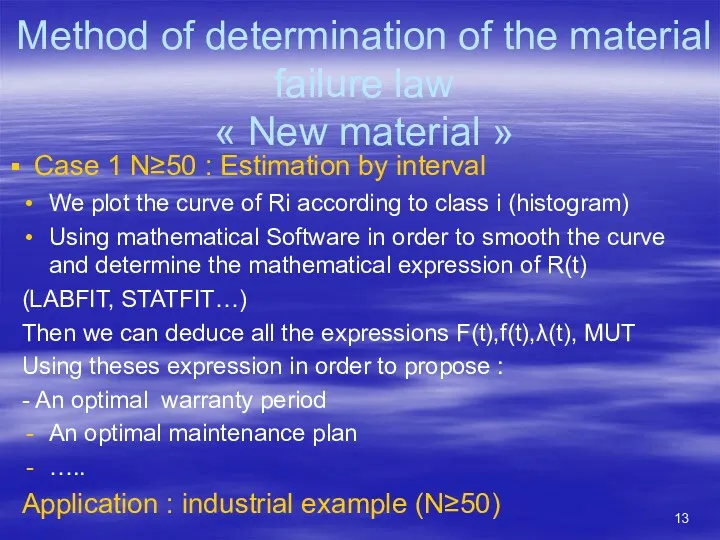
Case 1 N≥50
Method of determination of the material failure law
« New material »
Case 1 N≥50
Method of determination of the material failure law
« New material »
Case 1 N≥50
Method of determination of the material failure law
« New material »
Case 1 N≥50
Method of determination of the material failure law
« New material »
Case 1 N≥50
Method of determination of the material failure law
« New material »
Case 1 N≥50
Method of determination of the material failure law
« New material »
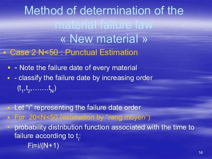
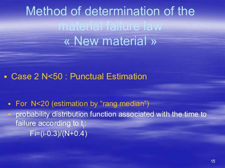
Case 2 N<50
Method of determination of the material failure law
« New material »
Case 2 N<50
Method of determination of the material failure law
« New material »
Case 2 N<50
Method of determination of the material failure law
« New material »
Case 2 N<50
Method of determination of the material failure law
« New material »
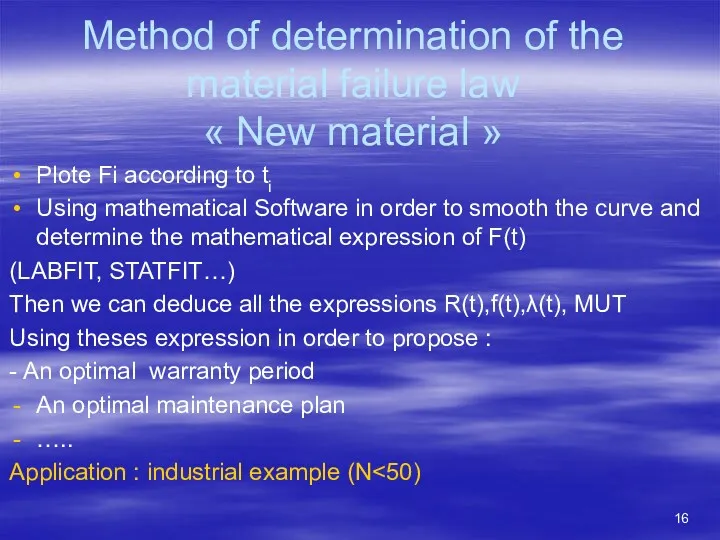
Plote Fi according
Method of determination of the material failure law
« New material »
Plote Fi according
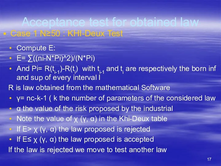
Acceptance test for obtained law
Case 1 N≥50 : KHI-Deux Test
Compute E:
Acceptance test for obtained law
Case 1 N≥50 : KHI-Deux Test
Compute E:
Acceptance test for obtained law
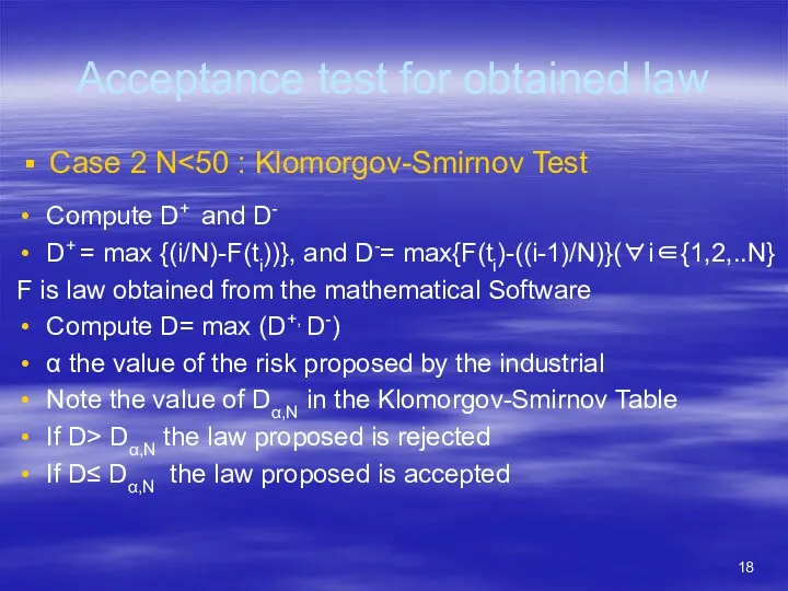
Case 2 N<50 : Klomorgov-Smirnov Test
Compute D+
Acceptance test for obtained law
Case 2 N<50 : Klomorgov-Smirnov Test
Compute D+
Principal law used in industry and research in reliability frame
Principal law used in industry and research in reliability frame
Usuel discret law
Usuel discret law
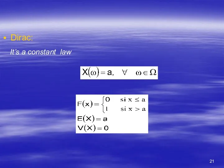
It’s a constant law
Dirac:
It’s a constant law
Dirac:
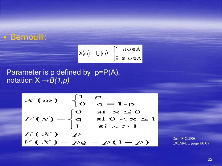
Bernoulli:
Parameter is p defined by p=P(A),
notation X →B(1,p)
Dem FIGURE EXEMPLE
Bernoulli:
Parameter is p defined by p=P(A),
notation X →B(1,p)
Dem FIGURE EXEMPLE
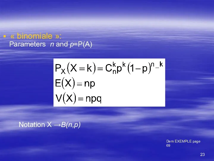
Parameters n and p=P(A)
« binomiale »:
Notation X →B(n,p)
Dem EXEMPLE page 69
Parameters n and p=P(A)
« binomiale »:
Notation X →B(n,p)
Dem EXEMPLE page 69
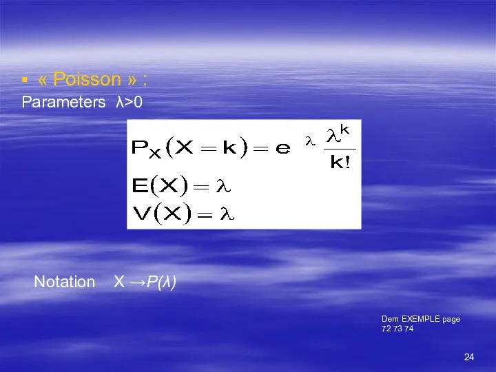
Parameters λ>0
« Poisson » :
Notation X →P(λ)
Dem EXEMPLE page 72 73 74
Parameters λ>0
« Poisson » :
Notation X →P(λ)
Dem EXEMPLE page 72 73 74
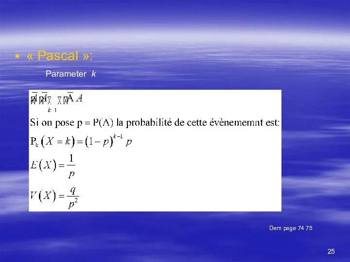
« Pascal »:
Dem page 74 75
Parameter k
« Pascal »:
Dem page 74 75
Parameter k
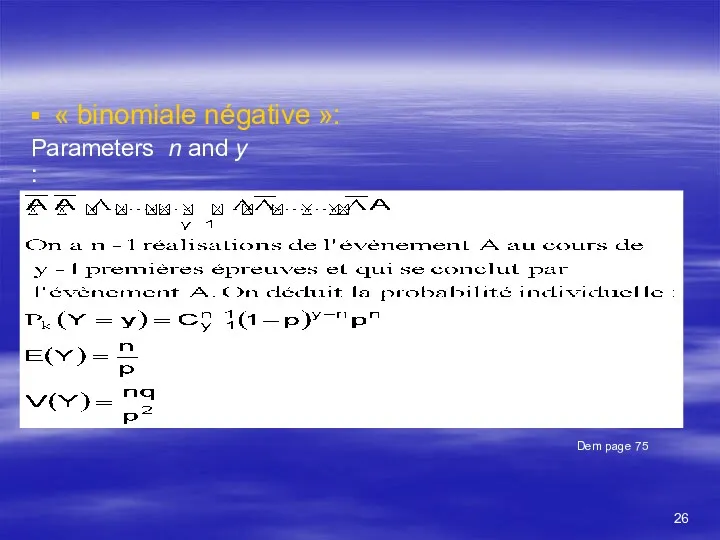
Parameters n and y
:
« binomiale négative »:
Dem page 75
Parameters n and y
:
« binomiale négative »:
Dem page 75
Continuous law
Dem page 77 78
Continuous law
Dem page 77 78
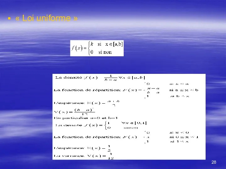
« Loi uniforme »
« Loi uniforme »
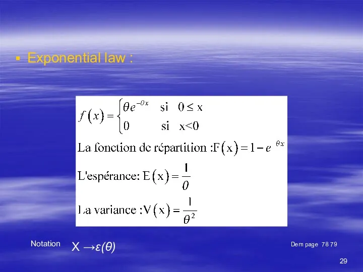
Exponential law :
Notation X →ε(θ)
Dem page 78 79
Exponential law :
Notation X →ε(θ)
Dem page 78 79
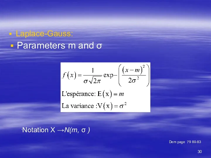
Laplace-Gauss:
.Notation X →N(m, σ )
Dem page 79 80-83
Parameters m and σ
Laplace-Gauss:
.Notation X →N(m, σ )
Dem page 79 80-83
Parameters m and σ
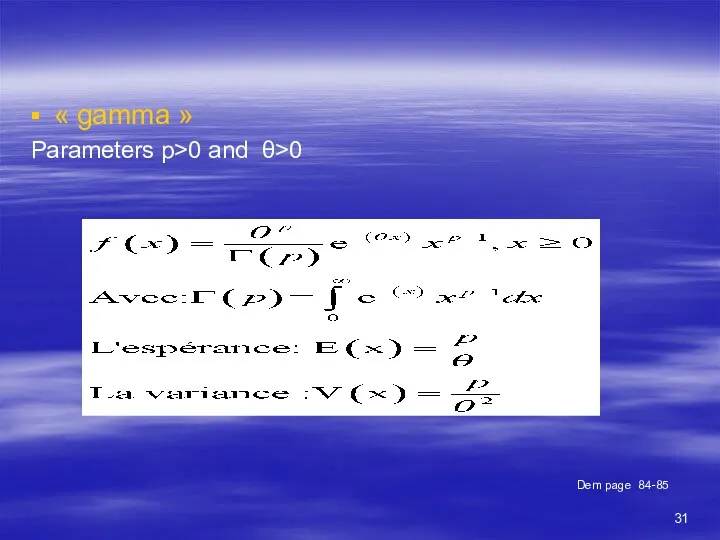
Parameters p>0 and θ>0
« gamma »
Dem page 84-85
Parameters p>0 and θ>0
« gamma »
Dem page 84-85
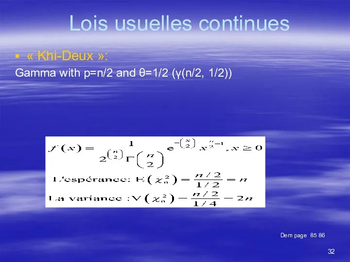
Lois usuelles continues
Gamma with p=n/2 and θ=1/2 (γ(n/2, 1/2))
« Khi-Deux »:
Dem page 85
Lois usuelles continues
Gamma with p=n/2 and θ=1/2 (γ(n/2, 1/2))
« Khi-Deux »:
Dem page 85
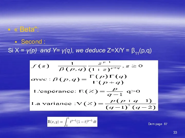
Si X = γ(p) and Y= γ(q), we deduce Z=X/Y =
Si X = γ(p) and Y= γ(q), we deduce Z=X/Y =
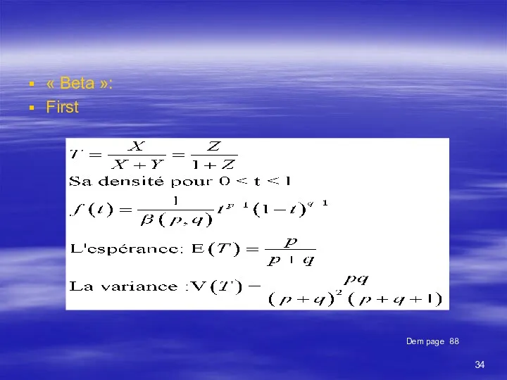
« Beta »:
First
Dem page 88
« Beta »:
First
Dem page 88
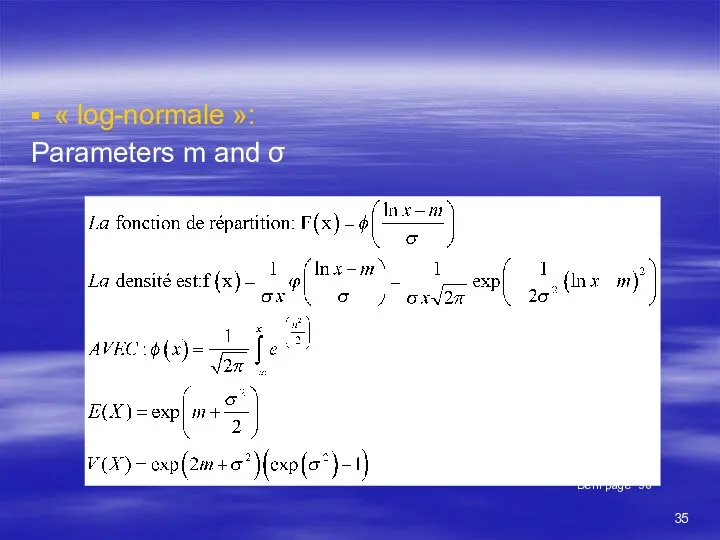
Parameters m and σ
« log-normale »:
Dem page 90
Parameters m and σ
« log-normale »:
Dem page 90
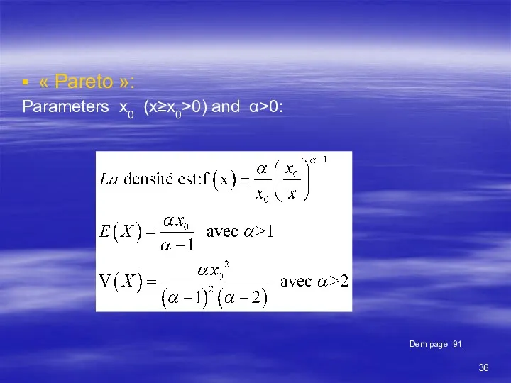
Parameters x0 (x≥x0>0) and α>0:
« Pareto »:
Dem page 91
Parameters x0 (x≥x0>0) and α>0:
« Pareto »:
Dem page 91
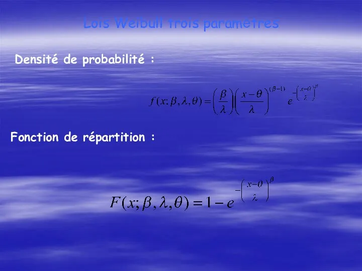
Lois Weibull trois paramètres
Densité de probabilité :
Fonction de répartition :
Lois Weibull trois paramètres
Densité de probabilité :
Fonction de répartition :
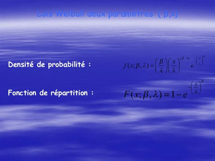
Lois Weibull deux paramètres ( β,λ)
Densité de probabilité :
Fonction de répartition
Lois Weibull deux paramètres ( β,λ)
Densité de probabilité :
Fonction de répartition
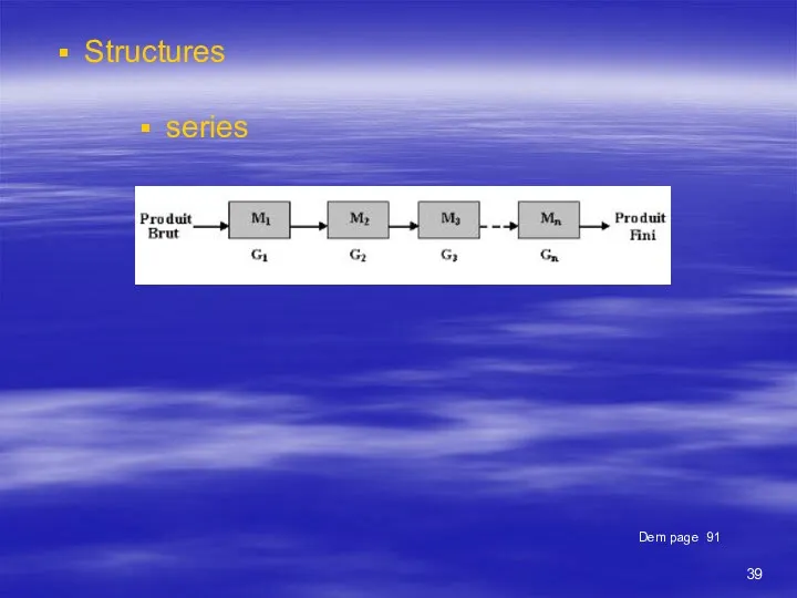
Structures
Dem page 91
series
Structures
Dem page 91
series
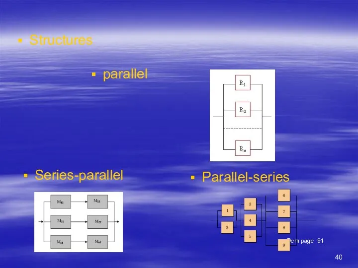
Structures
Dem page 91
parallel
Series-parallel
Parallel-series
Structures
Dem page 91
parallel
Series-parallel
Parallel-series
Complex Structures
Bridge system
Dem page 91
Theorem of Bays
Exampl
Complex Structures
Bridge system
Dem page 91
Theorem of Bays
Exampl
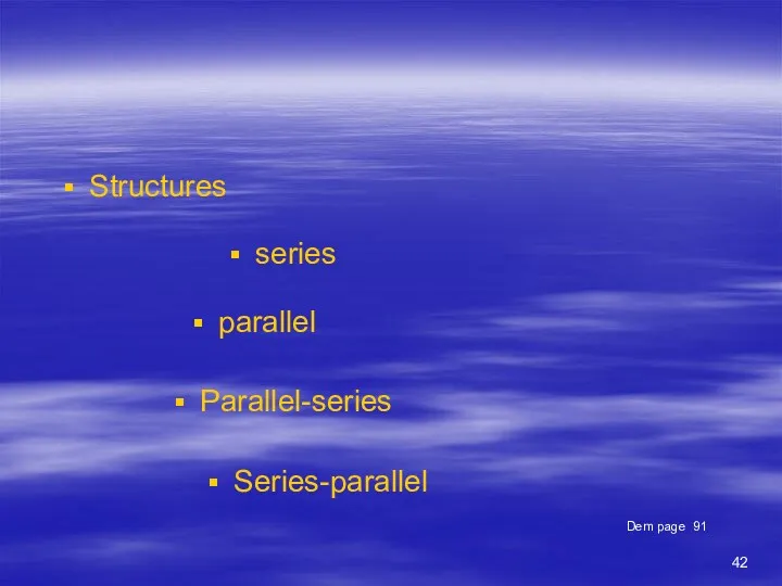
Structures
Dem page 91
series
parallel
Parallel-series
Series-parallel
Structures
Dem page 91
series
parallel
Parallel-series
Series-parallel

Structures
Dem page 91
series
parallel
Parallel-series
Series-parallel
Structures
Dem page 91
series
parallel
Parallel-series
Series-parallel
 Механізм управління розвитком сучасного підприємства
 Постановка целей SMART
 Система методов управления
 Управление эффективностью компании
 Организация как функция управления
 Страхование жизни. Доконтрактное обучение. 3 день
 Классификация управленческих решений
 Выявление проблем и пути их устранения
 Концепции управления персоналом
 Методы определения качественной потребности в персонале
 Организующая схема компании. Семинары по управлению
 Nextlevel. Трансформационный тренинг
 Премия качества Деминга
 Лидерство и стили управления
 Внутрифирменный кодекс корпоративной этики
 Основы предпринимательской деятельности
 Виды и методы обучения персонала в организации
 Стратегия управления персоналом
 Обучение новых сотрудников
 Планування часу
 Менеджмент в здравоохранении
 Измерение, анализ, улучшение
 Мотивация и стимулирование персонала в организации ООО Альфа Транс Терминал
 Управление проектами Agile и Scrum
 Совершенствование методов оценки сотрудников государственного учреждения
 Стратегічне планування в публічному управлінні
 Регламентация и нормирование труда
 Общий менеджмент. Постановка целей и z планирование в организации