- Empirical tools

Содержание
- 2. THE IMPORTANT DISTINCTION BETWEEN CORRELATION AND CAUSATION There are many examples where causation and correlation get
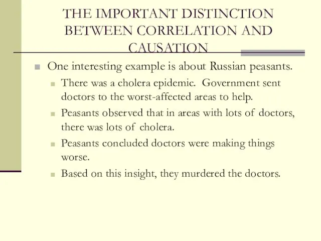
- 3. THE IMPORTANT DISTINCTION BETWEEN CORRELATION AND CAUSATION One interesting example is about Russian peasants. There was
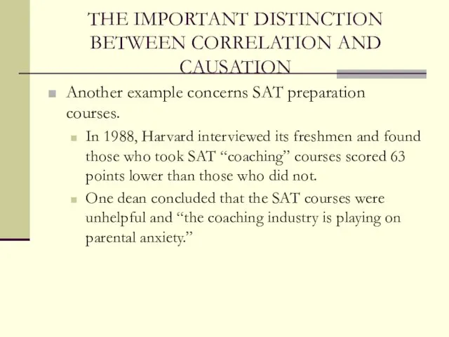
- 4. THE IMPORTANT DISTINCTION BETWEEN CORRELATION AND CAUSATION Another example concerns SAT preparation courses. In 1988, Harvard
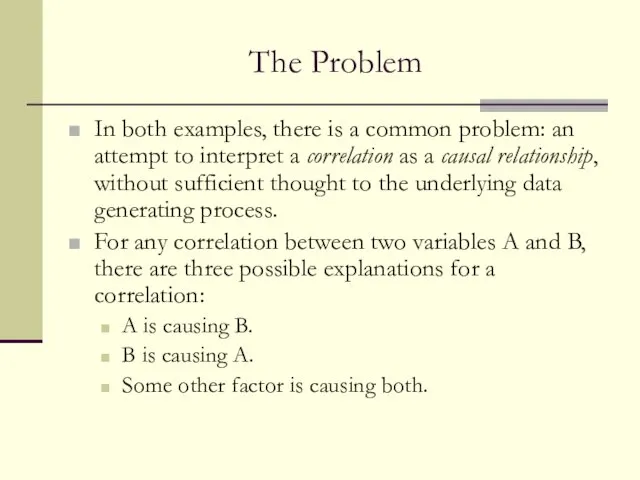
- 5. The Problem In both examples, there is a common problem: an attempt to interpret a correlation
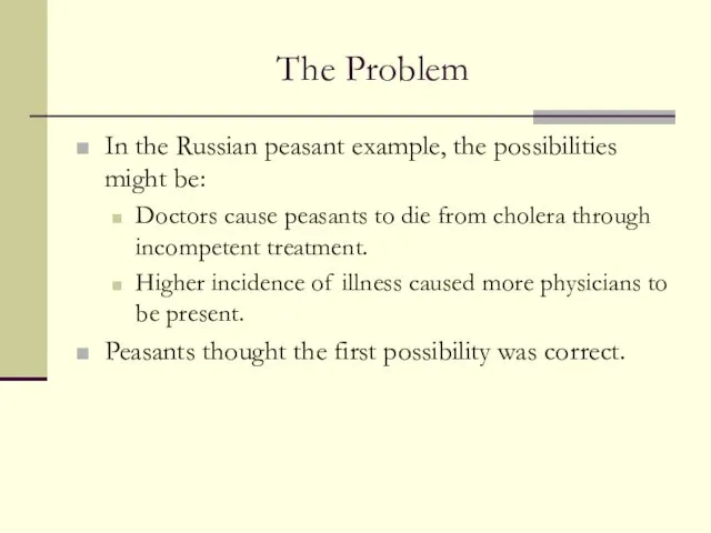
- 6. The Problem In the Russian peasant example, the possibilities might be: Doctors cause peasants to die
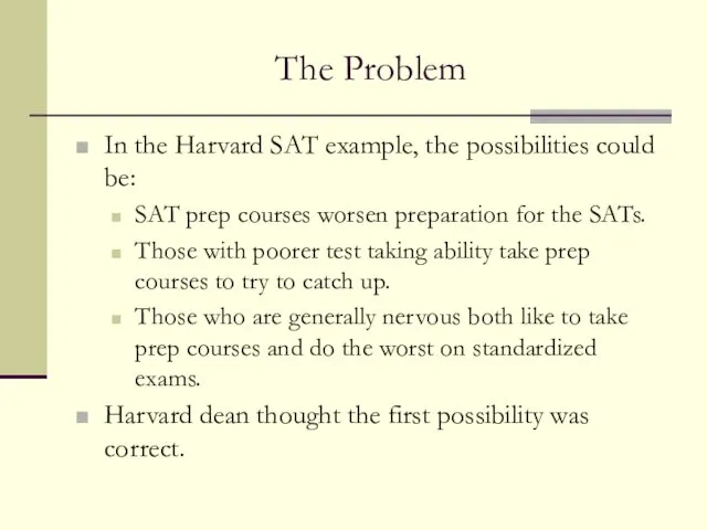
- 7. The Problem In the Harvard SAT example, the possibilities could be: SAT prep courses worsen preparation
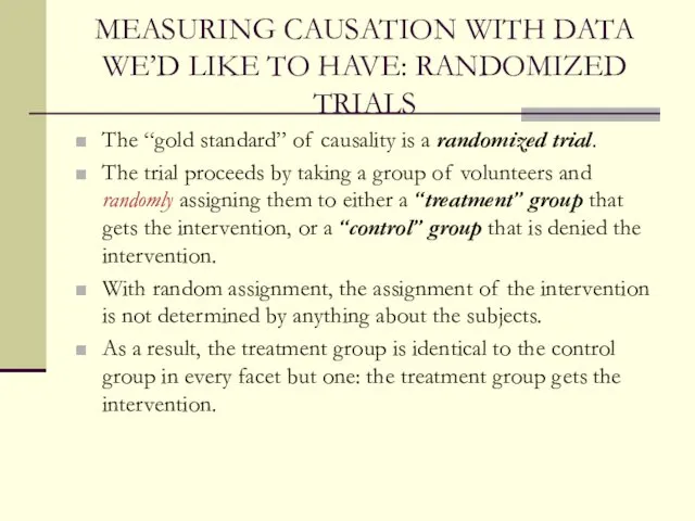
- 8. MEASURING CAUSATION WITH DATA WE’D LIKE TO HAVE: RANDOMIZED TRIALS The “gold standard” of causality is
- 9. Control vs Treatment groups. Randomness vs Biases. In the SAT example, the “treatment” group members are
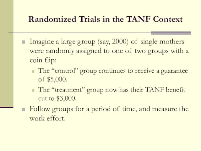
- 10. Randomized Trials in the TANF Context Imagine a large group (say, 2000) of single mothers were
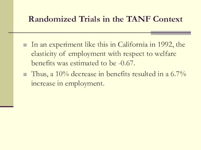
- 11. Randomized Trials in the TANF Context In an experiment like this in California in 1992, the
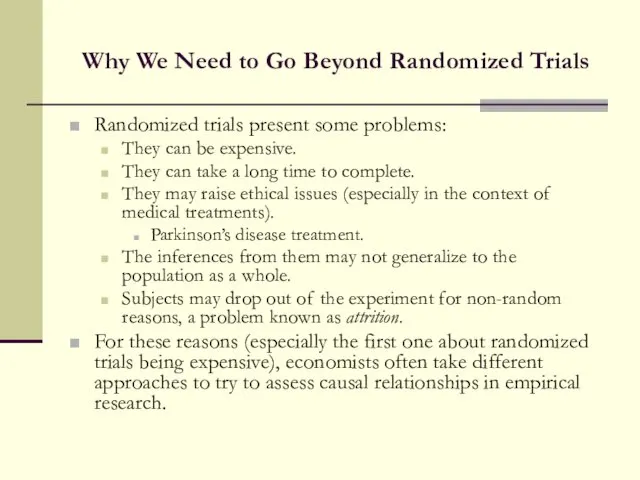
- 12. Why We Need to Go Beyond Randomized Trials Randomized trials present some problems: They can be
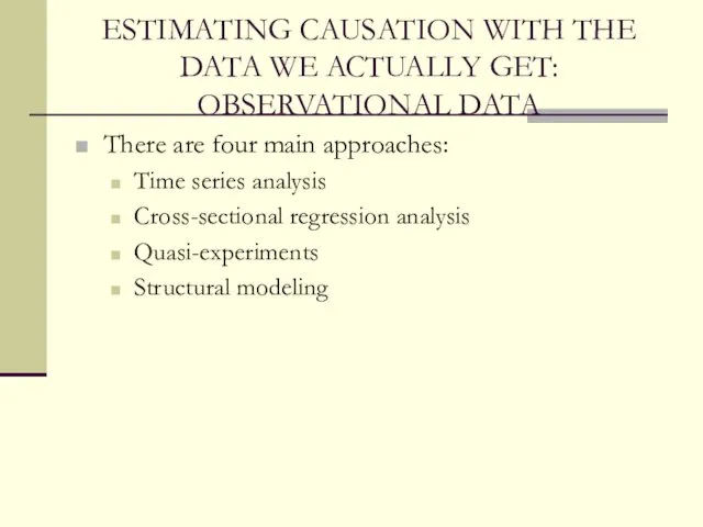
- 13. ESTIMATING CAUSATION WITH THE DATA WE ACTUALLY GET: OBSERVATIONAL DATA There are four main approaches: Time
- 15. Time Series Analysis Figure 1 reveals that real benefits have declined dramatically over time, while average
- 16. Time Series Analysis Many potential explanations for the changes, too, such as: Greater acceptance of women
- 17. Quasi-Experiments Quasi-experiments are changes in the economic environment that create roughly identical treatment and control groups
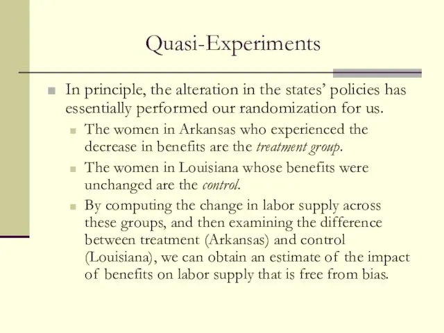
- 18. Quasi-Experiments In principle, the alteration in the states’ policies has essentially performed our randomization for us.
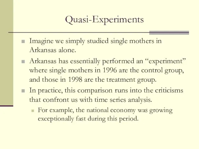
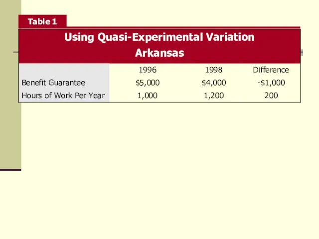
- 19. Quasi-Experiments Imagine we simply studied single mothers in Arkansas alone. Arkansas has essentially performed an “experiment”
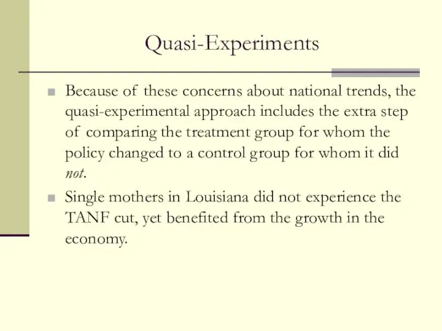
- 20. Quasi-Experiments Because of these concerns about national trends, the quasi-experimental approach includes the extra step of
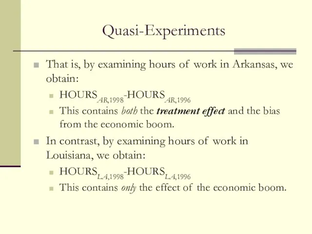
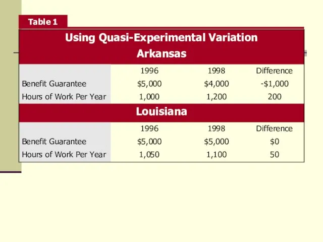
- 21. Quasi-Experiments That is, by examining hours of work in Arkansas, we obtain: HOURSAR,1998-HOURSAR,1996 This contains both
- 22. Quasi-Experiments By subtracting the change in hours of work in Louisiana from that in Arkansas, we
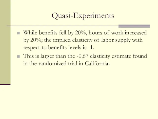
- 24. Quasi-Experiments While benefits fell by 20%, hours of work increased by 20%; the implied elasticity of
- 25. Quasi-Experiments There is likely to be bias in this “first-difference,” because there was major economic growth
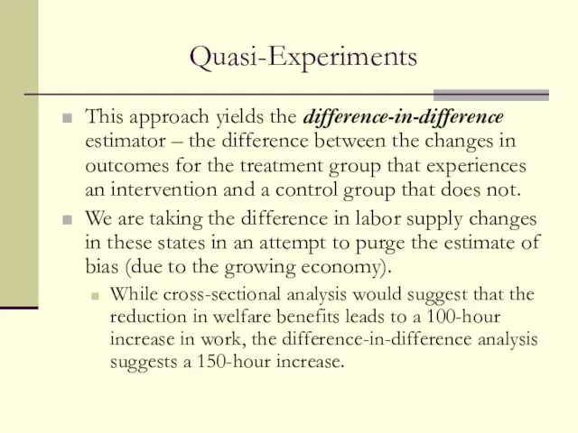
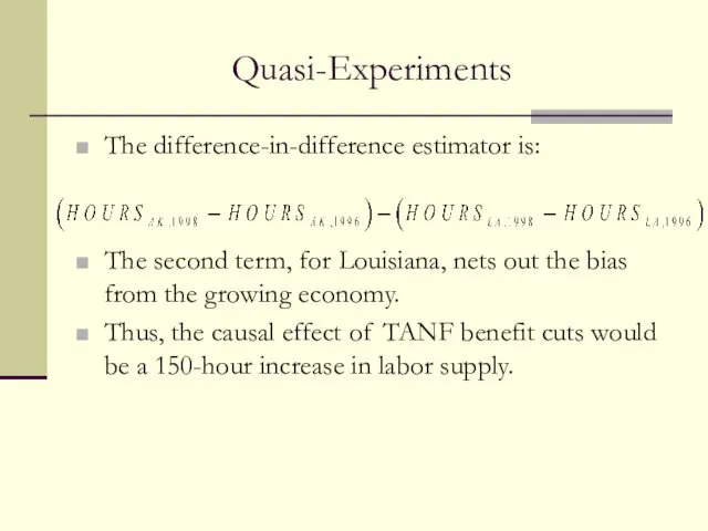
- 27. Quasi-Experiments This approach yields the difference-in-difference estimator – the difference between the changes in outcomes for
- 28. Quasi-Experiments The difference-in-difference estimator is: The second term, for Louisiana, nets out the bias from the
- 29. Quasi-Experiments: Problems with quasi-experimental analysis This approach also has problems, however. It is possible that the
- 30. Recap: trials of ERT ERT is the estrogen replacement therapy, which is a popular treatment for
- 32. Скачать презентацию
THE IMPORTANT DISTINCTION BETWEEN CORRELATION AND CAUSATION
There are many examples where
THE IMPORTANT DISTINCTION BETWEEN CORRELATION AND CAUSATION
There are many examples where
THE IMPORTANT DISTINCTION BETWEEN CORRELATION AND CAUSATION
One interesting example is about
THE IMPORTANT DISTINCTION BETWEEN CORRELATION AND CAUSATION
One interesting example is about
THE IMPORTANT DISTINCTION BETWEEN CORRELATION AND CAUSATION
Another example concerns SAT preparation
THE IMPORTANT DISTINCTION BETWEEN CORRELATION AND CAUSATION
Another example concerns SAT preparation
The Problem
In both examples, there is a common problem: an attempt
The Problem
In both examples, there is a common problem: an attempt
The Problem
In the Russian peasant example, the possibilities might be:
Doctors cause
The Problem
In the Russian peasant example, the possibilities might be:
Doctors cause
The Problem
In the Harvard SAT example, the possibilities could be:
SAT prep
The Problem
In the Harvard SAT example, the possibilities could be:
SAT prep
MEASURING CAUSATION WITH DATA WE’D LIKE TO HAVE: RANDOMIZED TRIALS
The “gold
MEASURING CAUSATION WITH DATA WE’D LIKE TO HAVE: RANDOMIZED TRIALS
The “gold
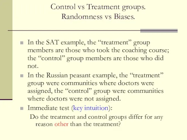
Control vs Treatment groups.
Randomness vs Biases.
In the SAT example, the “treatment”
Control vs Treatment groups.
Randomness vs Biases.
In the SAT example, the “treatment”
Randomized Trials in the TANF Context
Imagine a large group (say, 2000)
Randomized Trials in the TANF Context
Imagine a large group (say, 2000)
Randomized Trials in the TANF Context
In an experiment like this in
Randomized Trials in the TANF Context
In an experiment like this in
Why We Need to Go Beyond Randomized Trials
Randomized trials present some
Why We Need to Go Beyond Randomized Trials
Randomized trials present some
ESTIMATING CAUSATION WITH THE DATA WE ACTUALLY GET: OBSERVATIONAL DATA
There are
ESTIMATING CAUSATION WITH THE DATA WE ACTUALLY GET: OBSERVATIONAL DATA
There are
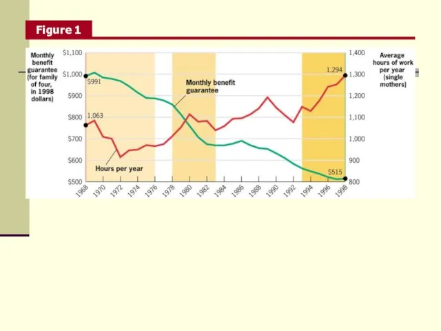
Time Series Analysis
Figure 1 reveals that real benefits have declined dramatically
Time Series Analysis
Figure 1 reveals that real benefits have declined dramatically
Time Series Analysis
Many potential explanations for the changes, too, such as:
Greater
Time Series Analysis
Many potential explanations for the changes, too, such as:
Greater
Quasi-Experiments
Quasi-experiments are changes in the economic environment that create roughly identical
Quasi-Experiments
Quasi-experiments are changes in the economic environment that create roughly identical
Quasi-Experiments
In principle, the alteration in the states’ policies has essentially performed
Quasi-Experiments
In principle, the alteration in the states’ policies has essentially performed
Quasi-Experiments
Imagine we simply studied single mothers in Arkansas alone.
Arkansas has essentially
Quasi-Experiments
Imagine we simply studied single mothers in Arkansas alone.
Arkansas has essentially
Quasi-Experiments
Because of these concerns about national trends, the quasi-experimental approach includes
Quasi-Experiments
Because of these concerns about national trends, the quasi-experimental approach includes
Quasi-Experiments
That is, by examining hours of work in Arkansas, we obtain:
HOURSAR,1998-HOURSAR,1996
This
Quasi-Experiments
That is, by examining hours of work in Arkansas, we obtain:
HOURSAR,1998-HOURSAR,1996
This
Quasi-Experiments
By subtracting the change in hours of work in Louisiana from
Quasi-Experiments
By subtracting the change in hours of work in Louisiana from
Quasi-Experiments
While benefits fell by 20%, hours of work increased by 20%;
Quasi-Experiments
While benefits fell by 20%, hours of work increased by 20%;
Quasi-Experiments
There is likely to be bias in this “first-difference,” because there
Quasi-Experiments
There is likely to be bias in this “first-difference,” because there
Quasi-Experiments
This approach yields the difference-in-difference estimator – the difference between the
Quasi-Experiments
This approach yields the difference-in-difference estimator – the difference between the
Quasi-Experiments
The difference-in-difference estimator is:
The second term, for Louisiana, nets out the
Quasi-Experiments
The difference-in-difference estimator is:
The second term, for Louisiana, nets out the
Quasi-Experiments:
Problems with quasi-experimental analysis
This approach also has problems, however.
It is possible
Quasi-Experiments:
Problems with quasi-experimental analysis
This approach also has problems, however.
It is possible
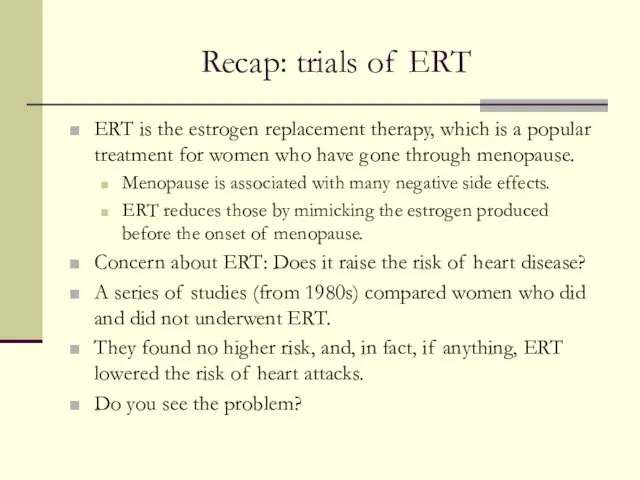
Recap: trials of ERT
ERT is the estrogen replacement therapy, which is
Recap: trials of ERT
ERT is the estrogen replacement therapy, which is
 Семья и брак
 Периодизация Д.Б. Бромлей
 Положение о совете молодых специалистов ООО Пермнефтеотдача
 Этнокультурные стереотипы и предрассудки
 Чрезвычайные ситуации социального характера (лекция 2)
 Становление российского парламентаризма
 Социальная инфраструктура
 Теория социального характера Рисмена
 Демографический анализ рождаемости, брачности и смертности: сущность, причины, основные показатели
 Отчет проекта Единая страна - доступная среда
 Введение в предметную область (описание ситуации как было)
 Гайк Маркосян. Предвыборная программа на пост председателя профкома
 Анализ поведения потребителей
 Социология как наука
 Стратегічний розвиток Дніпра
 Конфликт в межличностных отношениях,10 класс (профильный уровень)
 Права потребителей.
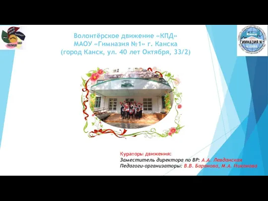 Волонтёрское движение КПД МАОУ Гимназия №1 г. Канска
 Отчёт председателя ученического совета город 112
 Социальная стратификация
 Международный день молодежи
 Мораль Моральные требования и представления
 Субкультура Хиппи
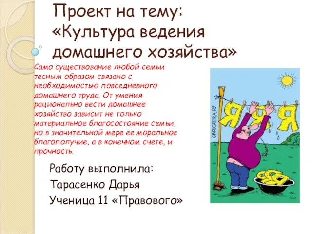 Культура ведения домашнего хозяйства
 Совет по творческому развитию студентов при Ректоре СВФУ имени М.К. Аммосова (СТР СВФУ)
 Коррупция и ее виды
 Актуальные проблемы девиантного поведения несовершеннолетних и молодежи Часть 1. Историко-социологическая
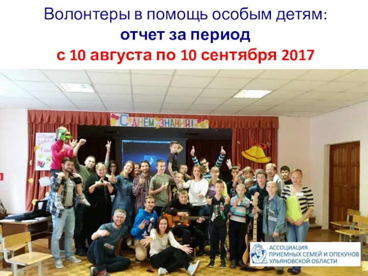 Волонтеры в помощь особым детям: отчет за период с 10 августа по 10 сентября 2017