- Neural Networks

Содержание
- 2. Pachshenko Galina Nikolaevna Associate Professor of Information System Department, Candidate of Technical Science
- 3. Week 3 Lecture 3
- 4. Topics Perceptron The perceptron learning algorithm Major components of a perceptron AND operator OR operator Neural
- 5. Machine Learning Classics: The Perceptron
- 6. Perceptron (Frank Rosenblatt, 1957) First learning algorithm for neural networks; Originally introduced for character classification, where
- 7. In machine learning, the perceptron is an algorithm for supervised learning of binary classifiers (functions that
- 8. The binary classifier defines that there should be only two categories for classification.
- 9. Classification is an example of supervised learning.
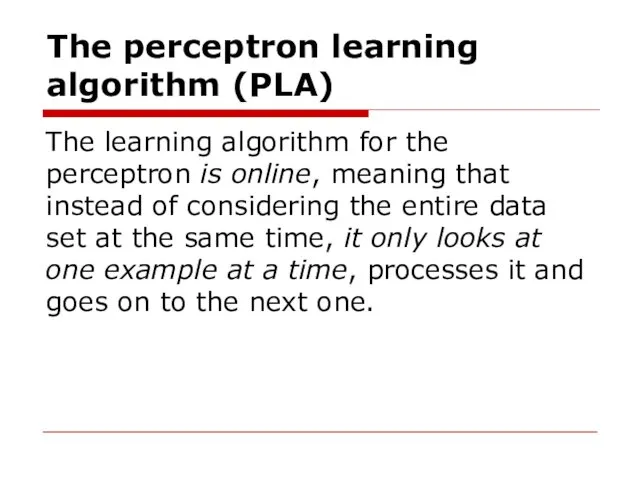
- 10. The perceptron learning algorithm (PLA) The learning algorithm for the perceptron is online, meaning that instead
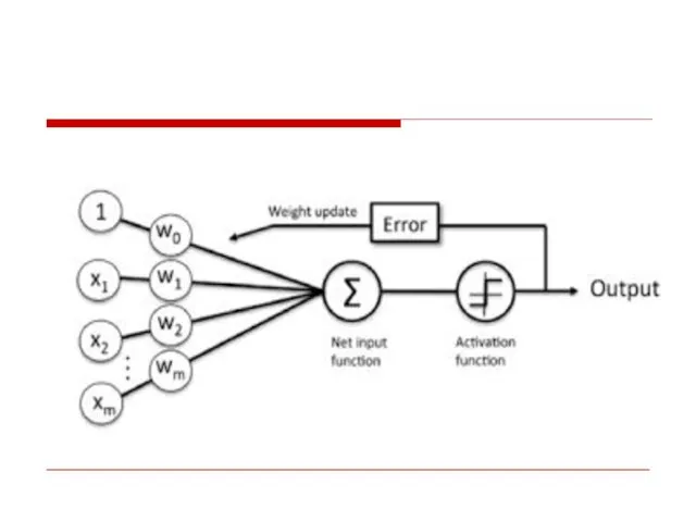
- 11. Following are the major components of a perceptron:
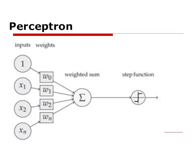
- 12. Input: All the features become the input for a perceptron. We denote the input of a
- 13. Weights: The values that are computed over the time of training the model. Initially, we start
- 14. Weighted summation: Weighted summation is the sum of the values that we get after the multiplication
- 15. Bias: A bias neuron allows a classifier to shift the decision boundary left or right. In
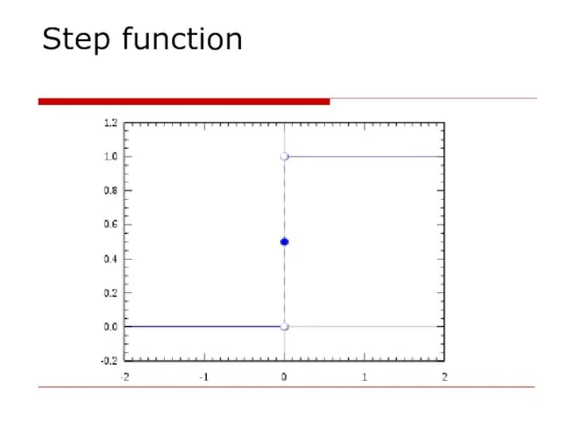
- 16. Step/activation function: The role of activation functions is to make neural networks nonlinear. For linear classification,
- 17. Output: The weighted summation is passed to the step/activation function and whatever value we get after
- 18. Inputs: 1 or 0
- 19. Outputs: 1 or 0
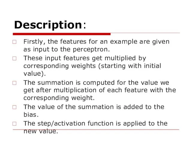
- 20. Description: Firstly, the features for an example are given as input to the perceptron. These input
- 21. Perceptron
- 22. Step function
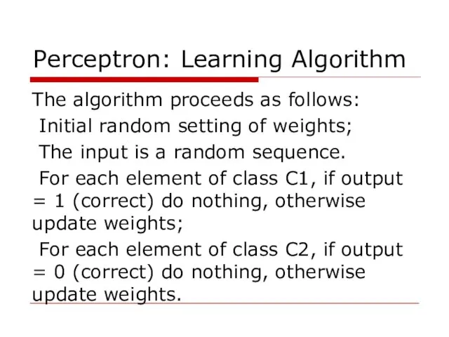
- 23. Perceptron: Learning Algorithm The algorithm proceeds as follows: Initial random setting of weights; The input is
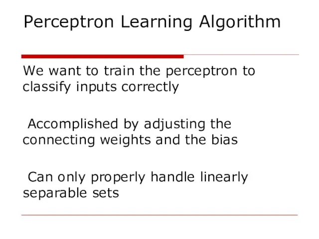
- 25. Perceptron Learning Algorithm We want to train the perceptron to classify inputs correctly Accomplished by adjusting
- 26. The perceptron is a machine learning algorithm used to determine whether an input belongs to one
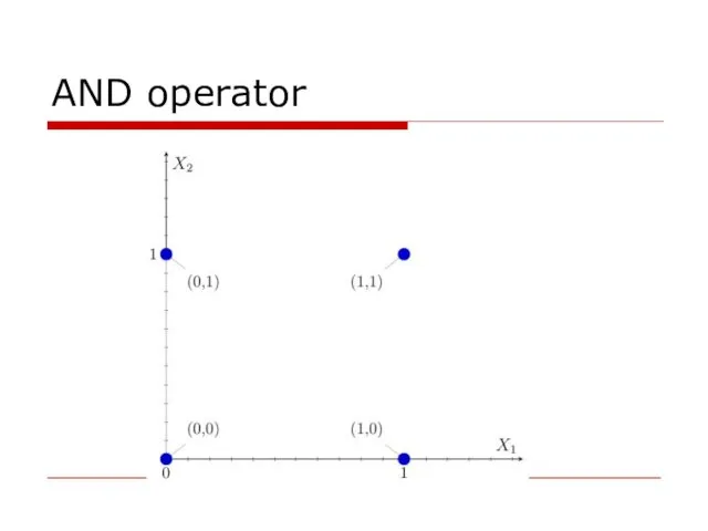
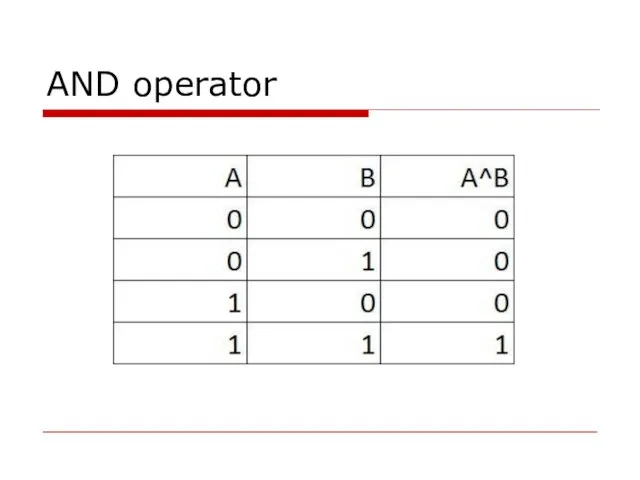
- 27. AND operator
- 28. AND operator
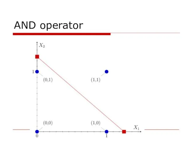
- 29. AND operator
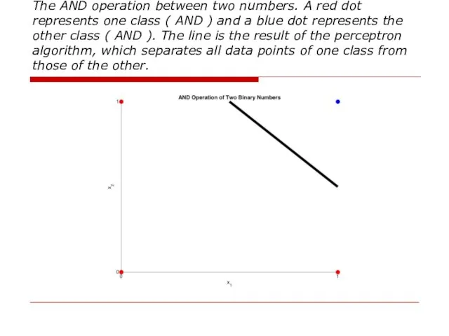
- 30. The AND operation between two numbers. A red dot represents one class ( AND ) and
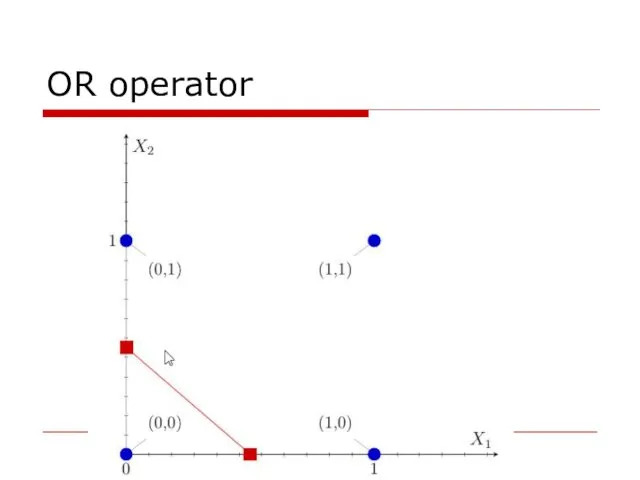
- 31. OR operator
- 32. OR operator
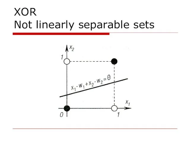
- 33. XOR Not linearly separable sets
- 34. XOR Not linearly separable sets
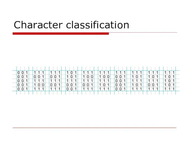
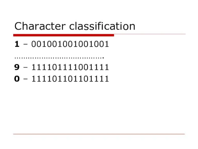
- 35. Character classification
- 36. Character classification 1 – 001001001001001 …………………………………. 9 – 111101111001111 0 – 111101101101111
- 37. Neural Network Learning Rules We know that, during ANN learning, to change the input/output behavior, we
- 38. Hebbian Learning Rule This rule, one of the oldest and simplest, was introduced by Donald Hebb
- 39. The Hebbian Learning Rule is a learning rule that specifies how much the weight of the
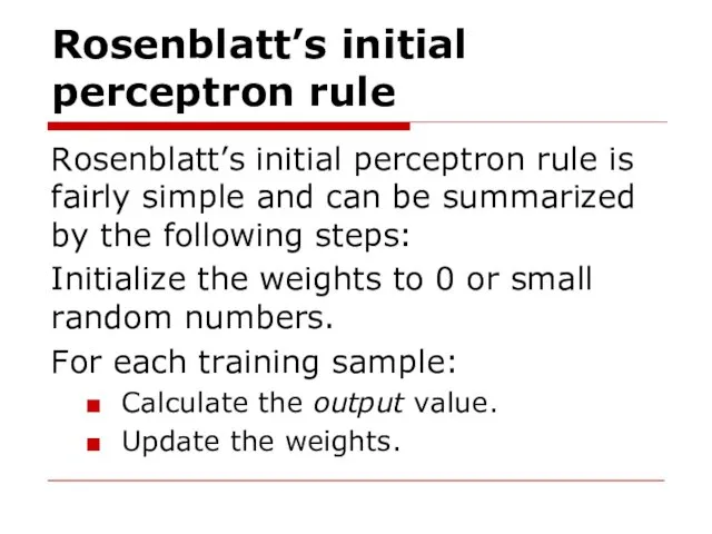
- 40. Rosenblatt’s initial perceptron rule Rosenblatt’s initial perceptron rule is fairly simple and can be summarized by
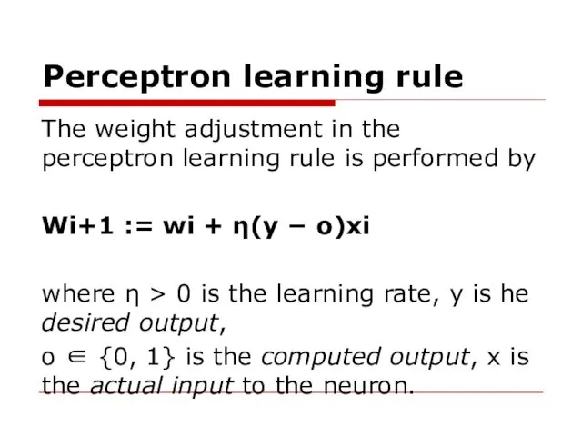
- 41. Perceptron learning rule The weight adjustment in the perceptron learning rule is performed by Wi+1 :=
- 42. Step 1 η > 0 is chosen, range [0,5; 0,7]. where η > 0 is the
- 43. Step 2 Weigts are initialized at small random values, The running error E is set to
- 44. Step 3 Training starts here. For each element of class C1, if output = 1 (correct)
- 45. Step 4 Weights are updated
- 46. Step 5 Cumulative cycle error is computed by adding the present error to initial error.
- 47. Step 6 If i
- 48. Step 7 The training cycle is completed. For errow E = 0 terminate the training session.
- 49. The output value is the class label predicted by the unit step function that we defined
- 50. The value for updating the weights at each increment is calculated by the learning rule
- 51. Hebbian learning rule – It identifies, how to modify the weights of nodes of a network.
- 53. Скачать презентацию

Pachshenko
Galina Nikolaevna
Associate Professor of Information System Department,
Galina Nikolaevna
Associate Professor of Information System Department,
Week 3
Lecture 3
Week 3
Lecture 3
Topics
Perceptron
The perceptron learning algorithm
Major components of a perceptron
AND operator
OR operator
Neural
Topics
Perceptron
The perceptron learning algorithm
Major components of a perceptron
AND operator
OR operator
Neural
Machine Learning Classics: The Perceptron
Machine Learning Classics: The Perceptron
Perceptron
(Frank Rosenblatt, 1957)
First learning algorithm for neural networks;
Originally introduced for
Perceptron
(Frank Rosenblatt, 1957)
First learning algorithm for neural networks;
Originally introduced for
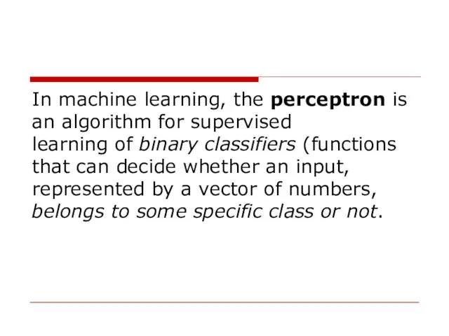
In machine learning, the perceptron is an algorithm for supervised learning of binary classifiers (functions that can decide
In machine learning, the perceptron is an algorithm for supervised learning of binary classifiers (functions that can decide
The binary classifier defines that there should be only two categories for classification.
The binary classifier defines that there should be only two categories for classification.
Classification is an example of supervised learning.
Classification is an example of supervised learning.
The perceptron learning algorithm (PLA)
The learning algorithm for the perceptron is
The perceptron learning algorithm (PLA)
The learning algorithm for the perceptron is
Following are the major components of a perceptron:
Following are the major components of a perceptron:
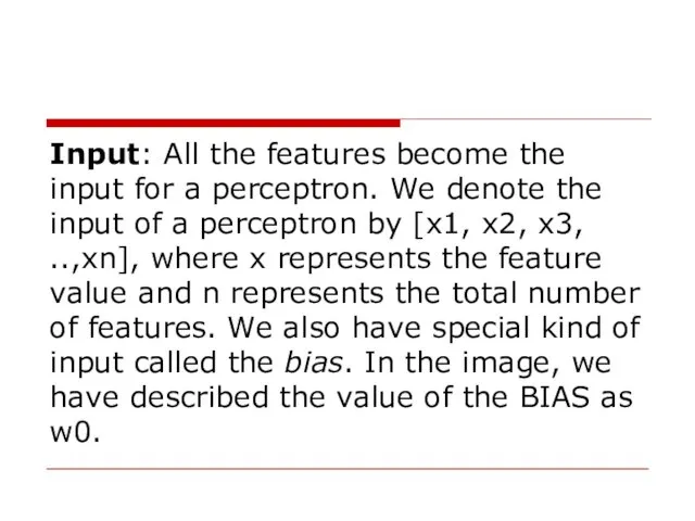
Input: All the features become the input for a perceptron. We denote
Input: All the features become the input for a perceptron. We denote
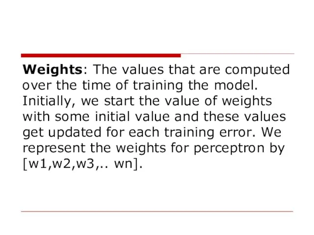
Weights: The values that are computed over the time of training the
Weights: The values that are computed over the time of training the
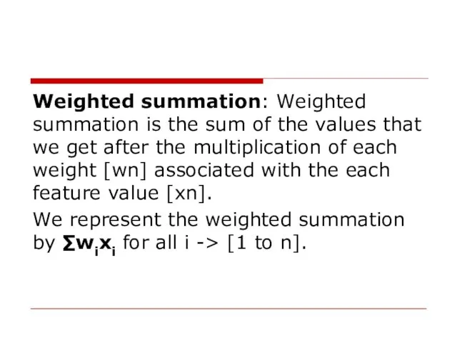
Weighted summation: Weighted summation is the sum of the values that
Weighted summation: Weighted summation is the sum of the values that
Bias: A bias neuron allows a classifier to shift the decision boundary
Bias: A bias neuron allows a classifier to shift the decision boundary
Step/activation function: The role of activation functions is to make neural
Step/activation function: The role of activation functions is to make neural
Output: The weighted summation is passed to the step/activation function and
Output: The weighted summation is passed to the step/activation function and
Inputs:
1 or 0
Inputs:
1 or 0
Outputs:
1 or 0
Outputs:
1 or 0
Description:
Firstly, the features for an example are given as input to
Description:
Firstly, the features for an example are given as input to
Perceptron
Perceptron
Step function
Step function
Perceptron: Learning Algorithm
The algorithm proceeds as follows:
Initial random setting
Perceptron: Learning Algorithm
The algorithm proceeds as follows:
Initial random setting
Perceptron Learning Algorithm
We want to train the perceptron to classify
Perceptron Learning Algorithm
We want to train the perceptron to classify
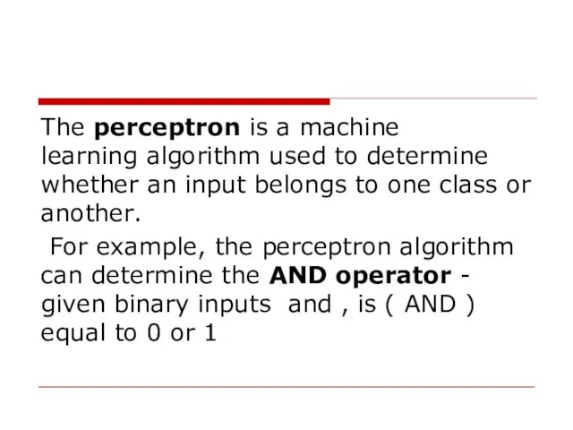
The perceptron is a machine learning algorithm used to determine whether an input belongs to one class or another.
For
The perceptron is a machine learning algorithm used to determine whether an input belongs to one class or another.
For
AND operator
AND operator
AND operator
AND operator
AND operator
AND operator
The AND operation between two numbers. A red dot represents one
The AND operation between two numbers. A red dot represents one
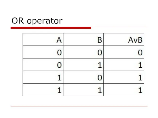
OR operator
OR operator
OR operator
OR operator
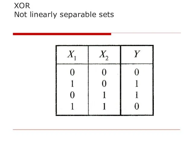
XOR
Not linearly separable sets
XOR
Not linearly separable sets
XOR
Not linearly separable sets
XOR
Not linearly separable sets
Character classification
Character classification
Character classification
1 – 001001001001001
………………………………….
9 – 111101111001111
0 – 111101101101111
Character classification
1 – 001001001001001
………………………………….
9 – 111101111001111
0 – 111101101101111
Neural Network Learning Rules
We know that, during ANN learning, to change
Neural Network Learning Rules
We know that, during ANN learning, to change
Hebbian Learning Rule
This rule, one of the oldest and simplest, was
Hebbian Learning Rule
This rule, one of the oldest and simplest, was
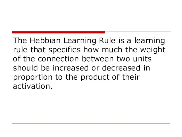
The Hebbian Learning Rule is a learning rule that specifies how
The Hebbian Learning Rule is a learning rule that specifies how
Rosenblatt’s initial perceptron rule
Rosenblatt’s initial perceptron rule is fairly simple and
Rosenblatt’s initial perceptron rule
Rosenblatt’s initial perceptron rule is fairly simple and
Perceptron learning rule
The weight adjustment in the perceptron learning rule is
Perceptron learning rule
The weight adjustment in the perceptron learning rule is
![Step 1 η > 0 is chosen, range [0,5; 0,7].](/_ipx/f_webp&q_80&fit_contain&s_1440x1080/imagesDir/jpg/29450/slide-41.jpg)
Step 1 η > 0 is chosen, range [0,5; 0,7].
where
Step 1 η > 0 is chosen, range [0,5; 0,7].
where
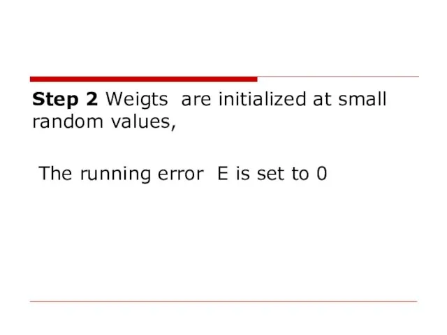
Step 2 Weigts are initialized at small random values,
The running
Step 2 Weigts are initialized at small random values,
The running
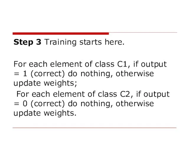
Step 3 Training starts here.
For each element of class C1, if
Step 3 Training starts here.
For each element of class C1, if
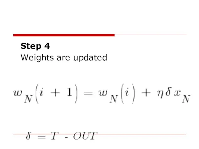
Step 4
Weights are updated
Step 4
Weights are updated
Step 5 Cumulative cycle error is computed by adding the present
Step 5 Cumulative cycle error is computed by adding the present
Step 6
If i < N then i := i +
Step 6
If i < N then i := i +
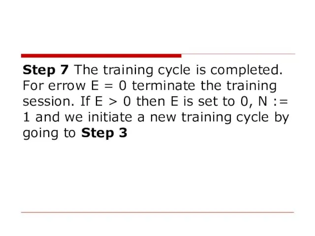
Step 7 The training cycle is completed. For errow E =
Step 7 The training cycle is completed. For errow E =
The output value is the class label predicted by the unit
The output value is the class label predicted by the unit
The value for updating the weights at each increment is calculated
The value for updating the weights at each increment is calculated
Hebbian learning rule – It identifies, how to modify the weights of
Hebbian learning rule – It identifies, how to modify the weights of
 Позиционирование ампайров и винг-ампайров в матчевых гонках (Umpires’ Positioning)
 Основи побудови радіоелектронної техніки. Загальні відомості про РЛС 19Ж6. (Тема 10.1)
 Транспортная безопасность
 Великая отечественная война
 Кузбасс: вчера. сегодня, завтра
 Паркувальний радар
 Презентация Права ребёнка
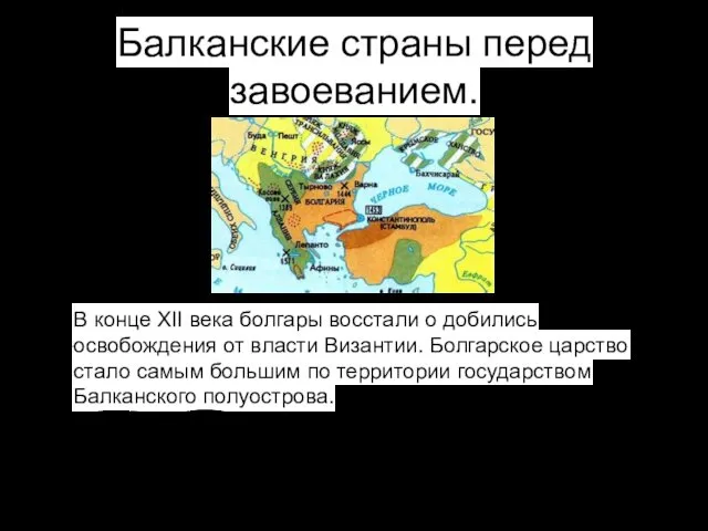 Балканские страны перед завоеванием
 Организационная перестройка по Дж. Коттеру
 Становление Древнерусского государства и правление первых русских князей
 Случаи вычитания 17 - 18 -
 Работа для участия в НПК Начальные классы (2 класс) - 1 место на школьном этапе, 2 - на районном.
 Призентация к интерактивному уроку:Основные классы неорганических соединений 7класс
 Презентация В память о Беслане
 Конструкция бесстыкового пути
 Василий Иванович Белов
 Подарочные наборы iPapai
 Башлангыч сыйныфта татар теленнән кагыйдәләр
 Площадь криволинейной трапеции
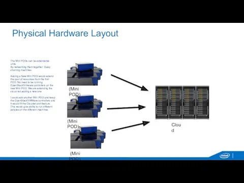 Physical Hardware Layout
 Организация работы станции Кая (Электрификация 8 и 9 путей)
 Природные уникумы Урала. Экологические проблемы Урала
 Valentines day riddles
 Буклет на звук Л
 История развития ГИС за рубежом и в нашей стране. Наиболее популярные современные ГИС. Их краткая характеристика
 Ручной труд как средство развития мелкой моторики
 Правовой стиль и правовые семьи по К. Цвайгерту и Х. Кётцу
 Биологическая роль липидов. Транспортные формы липидов