- Overview of data mining

Содержание
- 2. Outline Definition, motivation & application Branches of data mining Classification, clustering, Association rule mining Some classification
- 3. What Is Data Mining? Data mining (knowledge discovery in databases): Extraction of interesting (non-trivial, implicit, previously
- 4. Data Mining Definition Finding hidden information in a database Fit data to a model Similar terms
- 5. Motivation: Data explosion problem Automated data collection tools and mature database technology lead to tremendous amounts
- 6. Why Mine Data? Commercial Viewpoint Lots of data is being collected and warehoused Web data, e-commerce
- 7. Why Mine Data? Scientific Viewpoint Data collected and stored at enormous speeds (GB/hour) remote sensors on
- 8. Examples: What is (not) Data Mining? What is not Data Mining? Look up phone number in
- 9. Database Processing vs. Data Mining Processing Query Well defined SQL Query Poorly defined No precise query
- 10. Query Examples Database Data Mining Find all customers who have purchased milk Find all items which
- 11. Data Mining: Classification Schemes Decisions in data mining Kinds of databases to be mined Kinds of
- 12. Decisions in Data Mining Databases to be mined Relational, transactional, object-oriented, object-relational, active, spatial, time-series, text,
- 13. Data Mining Tasks Prediction Tasks Use some variables to predict unknown or future values of other
- 14. Data Mining Models and Tasks
- 15. Classification
- 16. Classification: Definition Given a collection of records (training set ) Each record contains a set of
- 17. An Example (from Pattern Classification by Duda & Hart & Stork – Second Edition, 2001) A
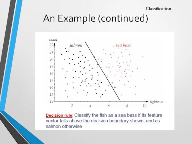
- 18. An Example (continued) Features (to distinguish): Length Lightness Width Position of mouth Classification
- 19. An Example (continued) Preprocessing: Images of different fishes are isolated from one another and from background;
- 20. An Example (continued) Domain knowledge: A sea bass is generally longer than a salmon Related feature:
- 21. An Example (continued) Classification model (hypothesis): The classifier generates a model from the training data to
- 22. An Example (continued) So the overall classification process goes like this ? Classification Preprocessing, and feature
- 23. An Example (continued) Classification Pre-processing, Feature extraction 12, salmon 15, sea bass 8, salmon 5, sea
- 24. An Example (continued) Why error? Insufficient training data Too few features Too many/irrelevant features Overfitting /
- 25. An Example (continued) Classification
- 26. An Example (continued) New Feature: Average lightness of the fish scales Classification
- 27. An Example (continued) Classification
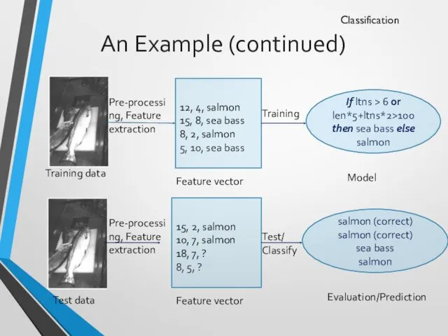
- 28. An Example (continued) Classification Pre-processing, Feature extraction 12, 4, salmon 15, 8, sea bass 8, 2,
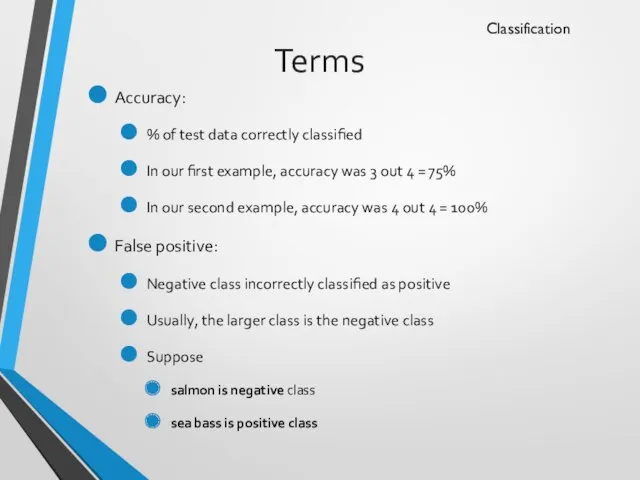
- 29. Terms Accuracy: % of test data correctly classified In our first example, accuracy was 3 out
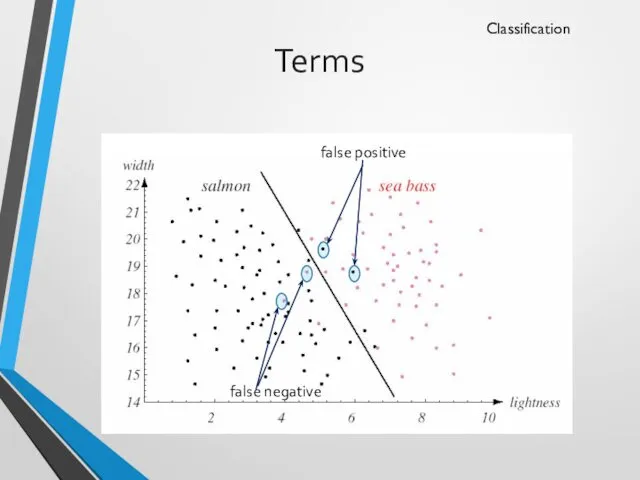
- 30. Terms Classification false positive false negative
- 31. Terms Cross validation (3 fold) Classification Testing Training Training Fold 2 Training Training Testing Fold 3
- 32. Classification Example 2 categorical categorical continuous class Training Set Learn Classifier
- 33. Classification: Application 1 Direct Marketing Goal: Reduce cost of mailing by targeting a set of consumers
- 34. Classification: Application 2 Fraud Detection Goal: Predict fraudulent cases in credit card transactions. Approach: Use credit
- 35. Classification: Application 3 Customer Attrition/Churn: Goal: To predict whether a customer is likely to be lost
- 36. Classification: Application 4 Sky Survey Cataloging Goal: To predict class (star or galaxy) of sky objects,
- 37. Classifying Galaxies Early Intermediate Late Data Size: 72 million stars, 20 million galaxies Object Catalog: 9
- 38. Clustering
- 39. Clustering Definition Given a set of data points, each having a set of attributes, and a
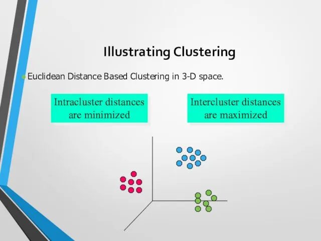
- 40. Illustrating Clustering Euclidean Distance Based Clustering in 3-D space. Intracluster distances are minimized Intercluster distances are
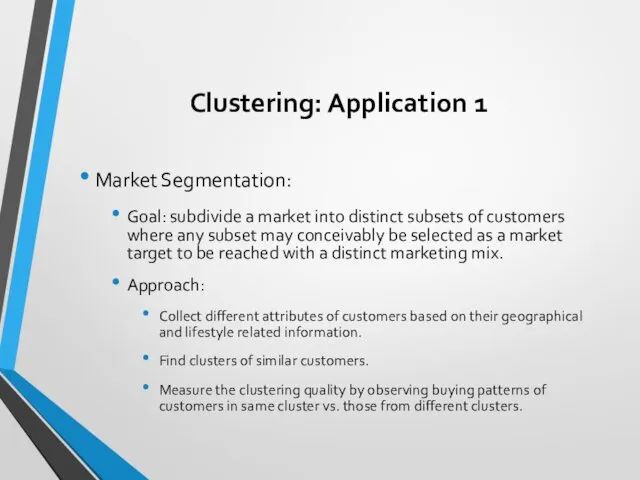
- 41. Clustering: Application 1 Market Segmentation: Goal: subdivide a market into distinct subsets of customers where any
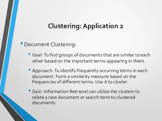
- 42. Clustering: Application 2 Document Clustering: Goal: To find groups of documents that are similar to each
- 43. Association rule mining
- 44. Association Rule Discovery: Definition Given a set of records each of which contain some number of
- 45. Association Rule Discovery: Application 1 Marketing and Sales Promotion: Let the rule discovered be {Bagels, …
- 46. Association Rule Discovery: Application 2 Supermarket shelf management. Goal: To identify items that are bought together
- 47. SOME Classification techniques
- 48. Bayes Theorem Posterior Probability: P(h1|xi) Prior Probability: P(h1) Bayes Theorem: Assign probabilities of hypotheses given a
- 49. Bayes Theorem Example Credit authorizations (hypotheses): h1=authorize purchase, h2 = authorize after further identification, h3=do not
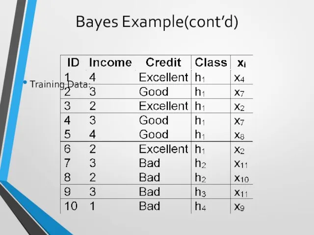
- 50. Bayes Example(cont’d) Training Data:
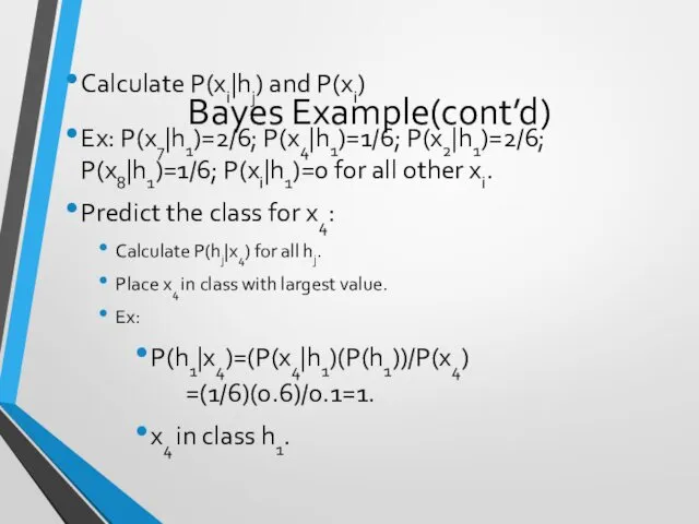
- 51. Bayes Example(cont’d) Calculate P(xi|hj) and P(xi) Ex: P(x7|h1)=2/6; P(x4|h1)=1/6; P(x2|h1)=2/6; P(x8|h1)=1/6; P(xi|h1)=0 for all other xi.
- 52. Hypothesis Testing Find model to explain behavior by creating and then testing a hypothesis about the
- 53. Chi Squared Statistic O – observed value E – Expected value based on hypothesis. Ex: O={50,93,67,78,87}
- 54. Regression Predict future values based on past values Linear Regression assumes linear relationship exists. y =
- 55. Linear Regression
- 56. Correlation Examine the degree to which the values for two variables behave similarly. Correlation coefficient r:
- 57. Similarity Measures Determine similarity between two objects. Similarity characteristics: Alternatively, distance measure measure how unlike or
- 58. Similarity Measures
- 59. Distance Measures Measure dissimilarity between objects
- 60. Twenty Questions Game
- 61. Decision Trees Decision Tree (DT): Tree where the root and each internal node is labeled with
- 62. Decision Tree Example
- 63. Decision Trees A Decision Tree Model is a computational model consisting of three parts: Decision Tree
- 64. Decision Tree Algorithm
- 65. DT Advantages/Disadvantages Advantages: Easy to understand. Easy to generate rules Disadvantages: May suffer from overfitting. Classifies
- 66. Neural Networks Based on observed functioning of human brain. (Artificial Neural Networks (ANN) Our view of
- 67. Neural Networks Neural Network (NN) is a directed graph F= with vertices V={1,2,…,n} and arcs A={
- 68. Neural Network Example
- 69. NN Node
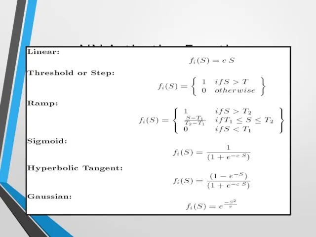
- 70. NN Activation Functions Functions associated with nodes in graph. Output may be in range [-1,1] or
- 71. NN Activation Functions
- 72. NN Learning Propagate input values through graph. Compare output to desired output. Adjust weights in graph
- 73. Neural Networks A Neural Network Model is a computational model consisting of three parts: Neural Network
- 74. NN Advantages Learning Can continue learning even after training set has been applied. Easy parallelization Solves
- 76. Скачать презентацию
Outline
Definition, motivation & application
Branches of data mining
Classification, clustering, Association rule mining
Some
Outline
Definition, motivation & application
Branches of data mining
Classification, clustering, Association rule mining
Some
What Is Data Mining?
Data mining (knowledge discovery in databases):
Extraction of interesting
What Is Data Mining?
Data mining (knowledge discovery in databases):
Extraction of interesting
Data Mining Definition
Finding hidden information in a database
Fit data to a
Data Mining Definition
Finding hidden information in a database
Fit data to a
Motivation:
Data explosion problem
Automated data collection tools and mature database
Motivation:
Data explosion problem
Automated data collection tools and mature database
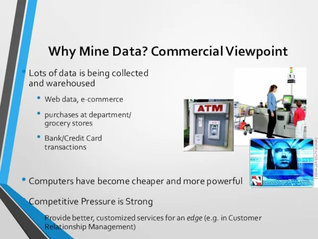
Why Mine Data? Commercial Viewpoint
Lots of data is being collected
and
Why Mine Data? Commercial Viewpoint
Lots of data is being collected and
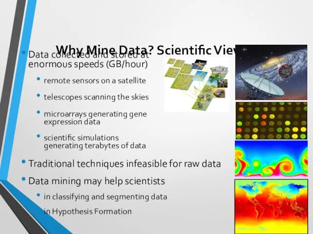
Why Mine Data? Scientific Viewpoint
Data collected and stored at
enormous speeds
Why Mine Data? Scientific Viewpoint
Data collected and stored at enormous speeds
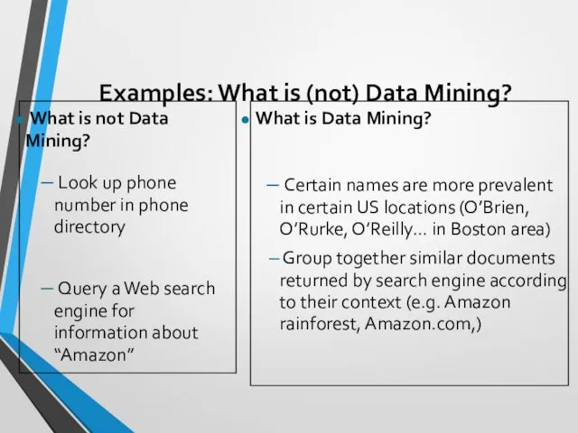
Examples: What is (not) Data Mining?
What is not Data Mining?
Examples: What is (not) Data Mining?
What is not Data Mining?
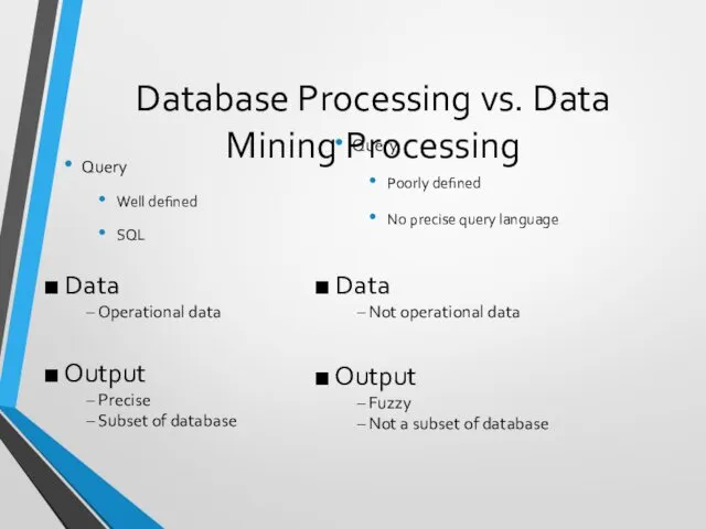
Database Processing vs. Data Mining Processing
Query
Well defined
SQL
Query
Poorly defined
No precise query language
Database Processing vs. Data Mining Processing
Query
Well defined
SQL
Query
Poorly defined
No precise query language
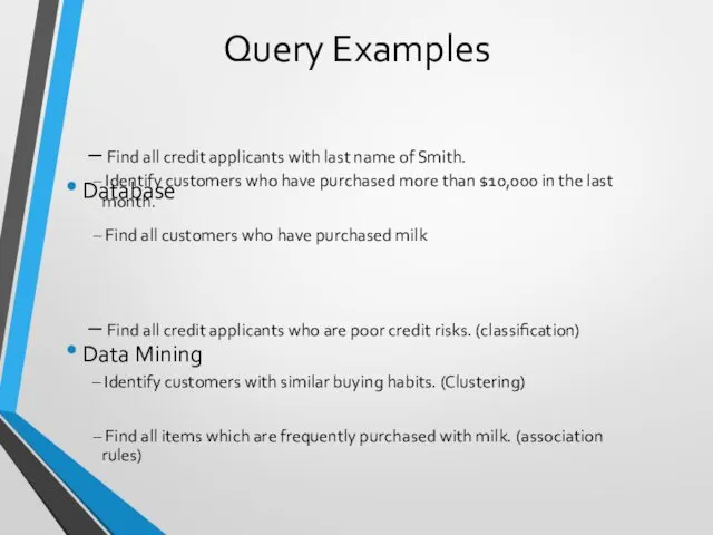
Query Examples
Database
Data Mining
Find all customers who have purchased milk
Find
Query Examples
Database
Data Mining
Find all customers who have purchased milk
Find
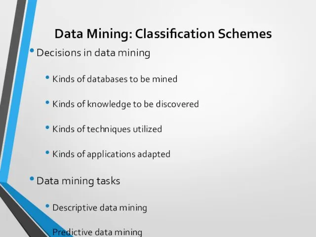
Data Mining: Classification Schemes
Decisions in data mining
Kinds of databases to be
Data Mining: Classification Schemes
Decisions in data mining
Kinds of databases to be
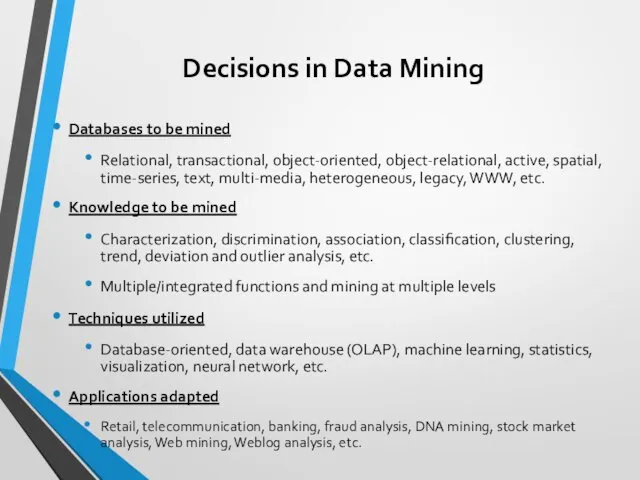
Decisions in Data Mining
Databases to be mined
Relational, transactional, object-oriented, object-relational, active,
Decisions in Data Mining
Databases to be mined
Relational, transactional, object-oriented, object-relational, active,
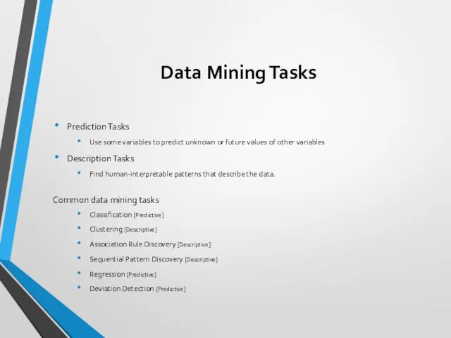
Data Mining Tasks
Prediction Tasks
Use some variables to predict unknown or future
Data Mining Tasks
Prediction Tasks
Use some variables to predict unknown or future
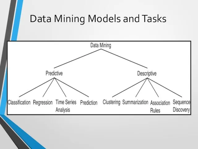
Data Mining Models and Tasks
Data Mining Models and Tasks

Classification
Classification
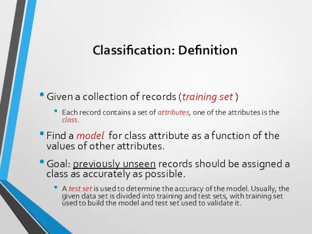
Classification: Definition
Given a collection of records (training set )
Each record contains
Classification: Definition
Given a collection of records (training set )
Each record contains
An Example
(from Pattern Classification by Duda & Hart & Stork –
An Example
(from Pattern Classification by Duda & Hart & Stork –
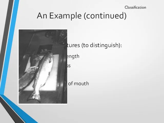
An Example (continued)
Features (to distinguish):
Length
Lightness
Width
Position of mouth
Classification
An Example (continued)
Features (to distinguish):
Length
Lightness
Width
Position of mouth
Classification
An Example (continued)
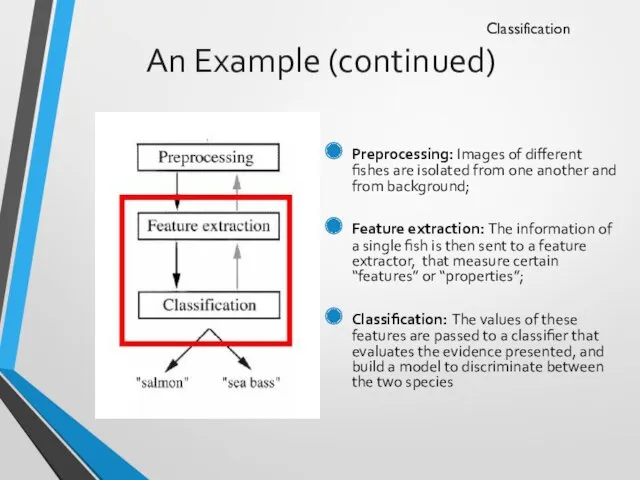
Preprocessing: Images of different fishes are isolated from one
An Example (continued)
Preprocessing: Images of different fishes are isolated from one
An Example (continued)
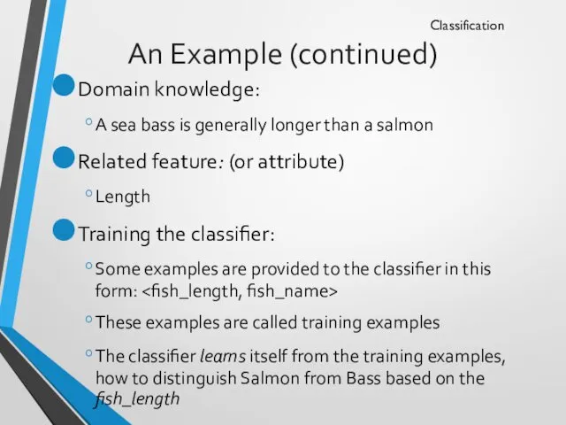
Domain knowledge:
A sea bass is generally longer than a
An Example (continued)
Domain knowledge:
A sea bass is generally longer than a
An Example (continued)
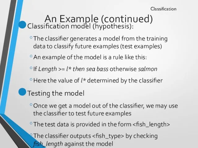
Classification model (hypothesis):
The classifier generates a model from the
An Example (continued)
Classification model (hypothesis):
The classifier generates a model from the
An Example (continued)
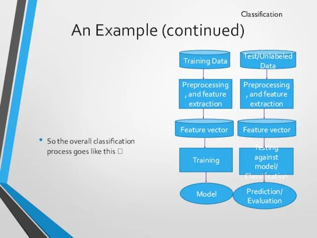
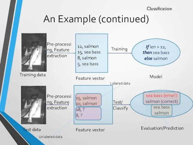
So the overall classification process goes like this ?
Classification
Preprocessing,
An Example (continued)
So the overall classification process goes like this ?
Classification
Preprocessing,
An Example (continued)
Classification
Pre-processing, Feature extraction
12, salmon
15, sea bass
8, salmon
5, sea bass
Training
An Example (continued)
Classification
Pre-processing, Feature extraction
12, salmon
15, sea bass
8, salmon
5, sea bass
Training
An Example (continued)
Why error?
Insufficient training data
Too few features
Too many/irrelevant features
Overfitting /
An Example (continued)
Why error?
Insufficient training data
Too few features
Too many/irrelevant features
Overfitting /
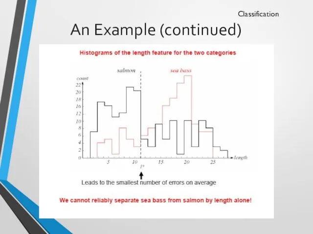
An Example (continued)
Classification
An Example (continued)
Classification
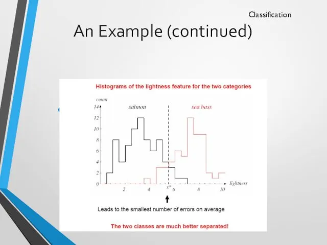
An Example (continued)
New Feature:
Average lightness of the fish scales
Classification
An Example (continued)
New Feature:
Average lightness of the fish scales
Classification
An Example (continued)
Classification
An Example (continued)
Classification
An Example (continued)
Classification
Pre-processing, Feature extraction
12, 4, salmon
15, 8, sea bass
8, 2,
An Example (continued)
Classification
Pre-processing, Feature extraction
12, 4, salmon
15, 8, sea bass
8, 2,
Terms
Accuracy:
% of test data correctly classified
In our first example, accuracy was
Terms
Accuracy:
% of test data correctly classified
In our first example, accuracy was
Terms
Classification
false positive
false negative
Terms
Classification
false positive
false negative
Terms
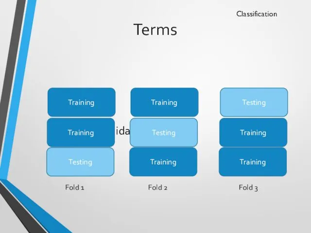
Cross validation (3 fold)
Classification
Testing
Training
Training
Fold 2
Training
Training
Testing
Fold 3
Training
Testing
Training
Fold 1
Terms
Cross validation (3 fold)
Classification
Testing
Training
Training
Fold 2
Training
Training
Testing
Fold 3
Training
Testing
Training
Fold 1
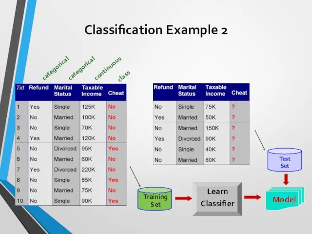
Classification Example 2
categorical
categorical
continuous
class
Training
Set
Learn
Classifier
Classification Example 2
categorical
categorical
continuous
class
Training
Set
Learn
Classifier
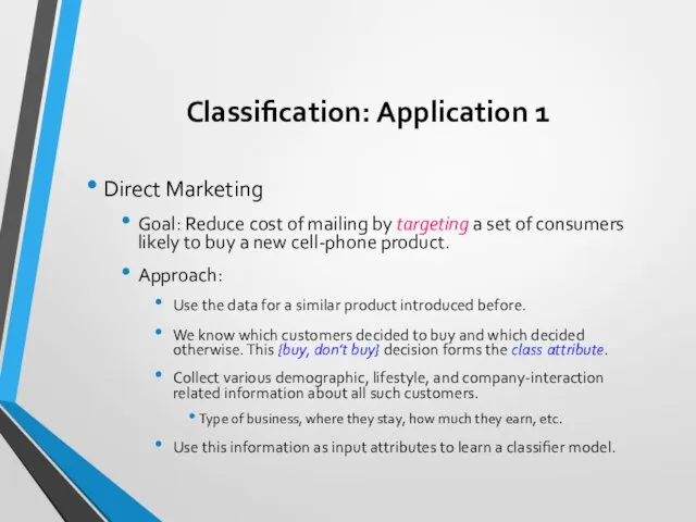
Classification: Application 1
Direct Marketing
Goal: Reduce cost of mailing by targeting a
Classification: Application 1
Direct Marketing
Goal: Reduce cost of mailing by targeting a
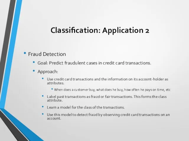
Classification: Application 2
Fraud Detection
Goal: Predict fraudulent cases in credit card transactions.
Approach:
Use
Classification: Application 2
Fraud Detection
Goal: Predict fraudulent cases in credit card transactions.
Approach:
Use
Classification: Application 3
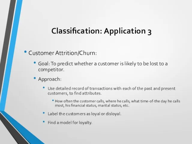
Customer Attrition/Churn:
Goal: To predict whether a customer is likely
Classification: Application 3
Customer Attrition/Churn:
Goal: To predict whether a customer is likely
Classification: Application 4
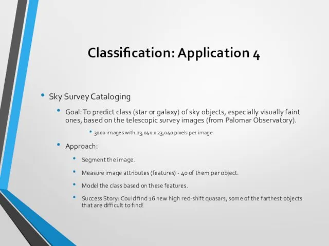
Sky Survey Cataloging
Goal: To predict class (star or galaxy)
Classification: Application 4
Sky Survey Cataloging
Goal: To predict class (star or galaxy)
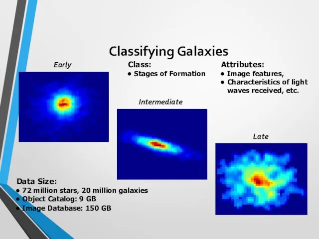
Classifying Galaxies
Early
Intermediate
Late
Data Size:
72 million stars, 20 million galaxies
Object Catalog: 9
Classifying Galaxies
Early
Intermediate
Late
Data Size:
72 million stars, 20 million galaxies
Object Catalog: 9

Clustering
Clustering
Clustering Definition
Given a set of data points, each having a set
Clustering Definition
Given a set of data points, each having a set
Illustrating Clustering
Euclidean Distance Based Clustering in 3-D space.
Intracluster distances
are minimized
Intercluster distances
are
Illustrating Clustering
Euclidean Distance Based Clustering in 3-D space.
Intracluster distances
are minimized
Intercluster distances
are
Clustering: Application 1
Market Segmentation:
Goal: subdivide a market into distinct subsets of
Clustering: Application 1
Market Segmentation:
Goal: subdivide a market into distinct subsets of
Clustering: Application 2
Document Clustering:
Goal: To find groups of documents that are
Clustering: Application 2
Document Clustering:
Goal: To find groups of documents that are

Association rule mining
Association rule mining
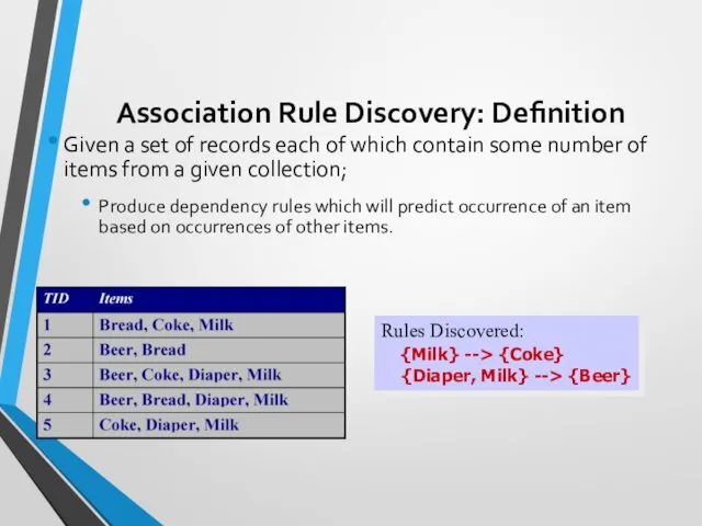
Association Rule Discovery: Definition
Given a set of records each of which
Association Rule Discovery: Definition
Given a set of records each of which
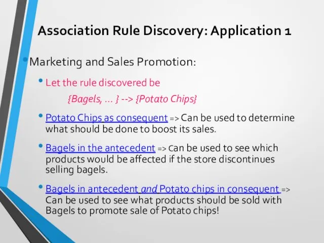
Association Rule Discovery: Application 1
Marketing and Sales Promotion:
Let the rule discovered
Association Rule Discovery: Application 1
Marketing and Sales Promotion:
Let the rule discovered
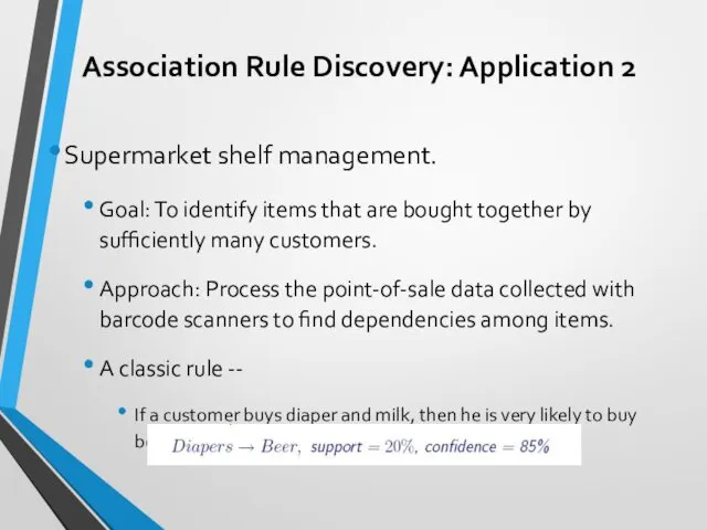
Association Rule Discovery: Application 2
Supermarket shelf management.
Goal: To identify items that
Association Rule Discovery: Application 2
Supermarket shelf management.
Goal: To identify items that

SOME Classification techniques
SOME Classification techniques
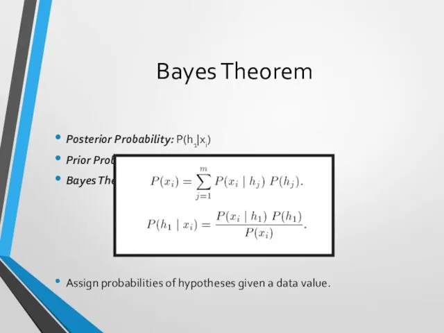
Bayes Theorem
Posterior Probability: P(h1|xi)
Prior Probability: P(h1)
Bayes Theorem:
Assign probabilities of hypotheses given
Bayes Theorem
Posterior Probability: P(h1|xi)
Prior Probability: P(h1)
Bayes Theorem:
Assign probabilities of hypotheses given
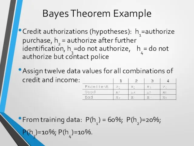
Bayes Theorem Example
Credit authorizations (hypotheses): h1=authorize purchase, h2 = authorize after
Bayes Theorem Example
Credit authorizations (hypotheses): h1=authorize purchase, h2 = authorize after
Bayes Example(cont’d)
Training Data:
Bayes Example(cont’d)
Training Data:
Bayes Example(cont’d)
Calculate P(xi|hj) and P(xi)
Ex: P(x7|h1)=2/6; P(x4|h1)=1/6; P(x2|h1)=2/6; P(x8|h1)=1/6; P(xi|h1)=0 for
Bayes Example(cont’d)
Calculate P(xi|hj) and P(xi)
Ex: P(x7|h1)=2/6; P(x4|h1)=1/6; P(x2|h1)=2/6; P(x8|h1)=1/6; P(xi|h1)=0 for
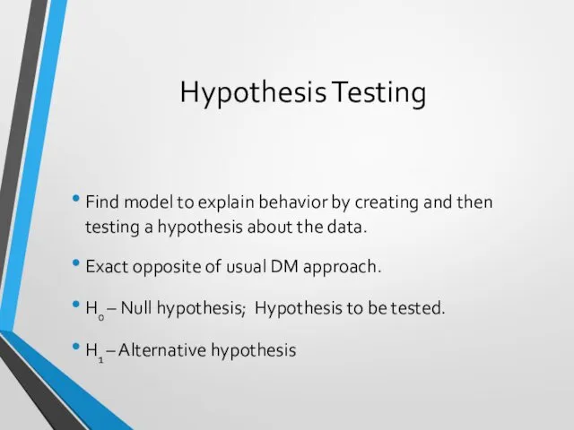
Hypothesis Testing
Find model to explain behavior by creating and then testing
Hypothesis Testing
Find model to explain behavior by creating and then testing
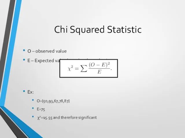
Chi Squared Statistic
O – observed value
E – Expected value based on
Chi Squared Statistic
O – observed value
E – Expected value based on
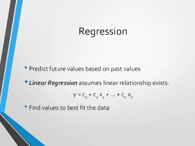
Regression
Predict future values based on past values
Linear Regression assumes linear relationship
Regression
Predict future values based on past values
Linear Regression assumes linear relationship
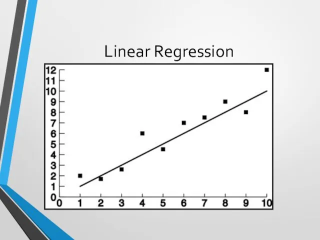
Linear Regression
Linear Regression
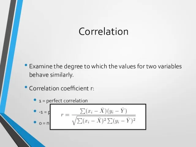
Correlation
Examine the degree to which the values for two variables behave
Correlation
Examine the degree to which the values for two variables behave
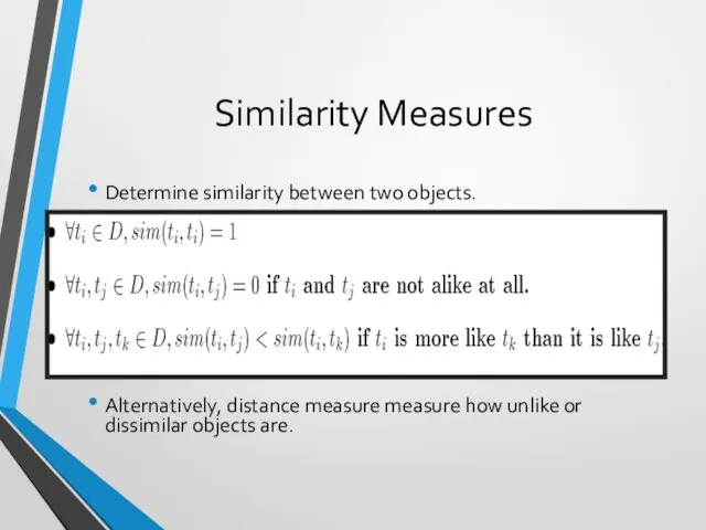
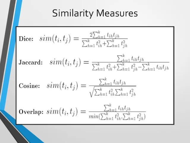
Similarity Measures
Determine similarity between two objects.
Similarity characteristics:
Alternatively, distance measure measure how
Similarity Measures
Determine similarity between two objects.
Similarity characteristics:
Alternatively, distance measure measure how
Similarity Measures
Similarity Measures
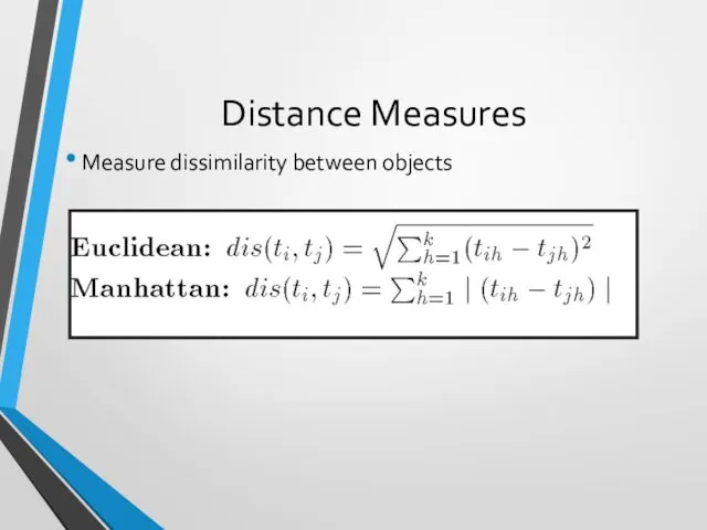
Distance Measures
Measure dissimilarity between objects
Distance Measures
Measure dissimilarity between objects
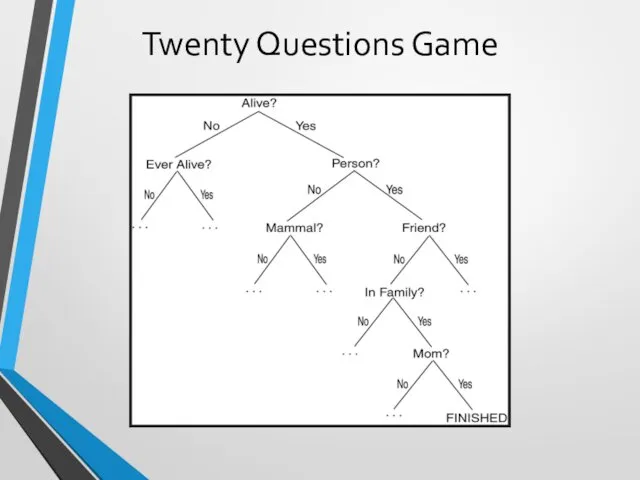
Twenty Questions Game
Twenty Questions Game
Decision Trees
Decision Tree (DT):
Tree where the root and each internal node
Decision Trees
Decision Tree (DT):
Tree where the root and each internal node
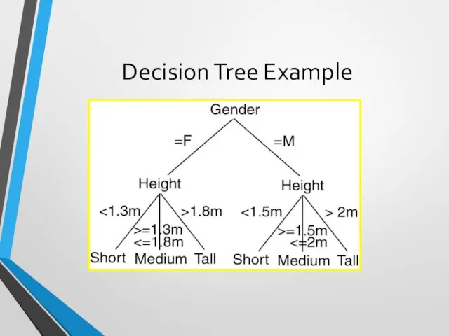
Decision Tree Example
Decision Tree Example
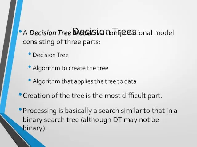
Decision Trees
A Decision Tree Model is a computational model consisting of
Decision Trees
A Decision Tree Model is a computational model consisting of
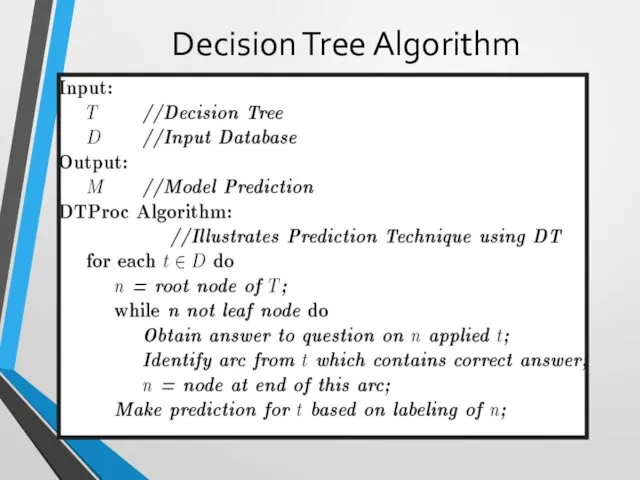
Decision Tree Algorithm
Decision Tree Algorithm
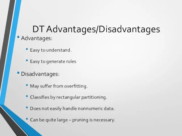
DT Advantages/Disadvantages
Advantages:
Easy to understand.
Easy to generate rules
Disadvantages:
May suffer from overfitting.
Classifies
DT Advantages/Disadvantages
Advantages:
Easy to understand.
Easy to generate rules
Disadvantages:
May suffer from overfitting.
Classifies
Neural Networks
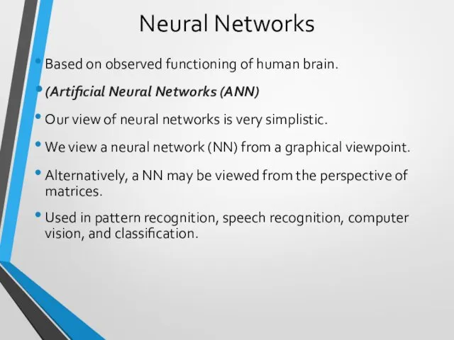
Based on observed functioning of human brain.
(Artificial Neural
Neural Networks
Based on observed functioning of human brain.
(Artificial Neural
Neural Networks
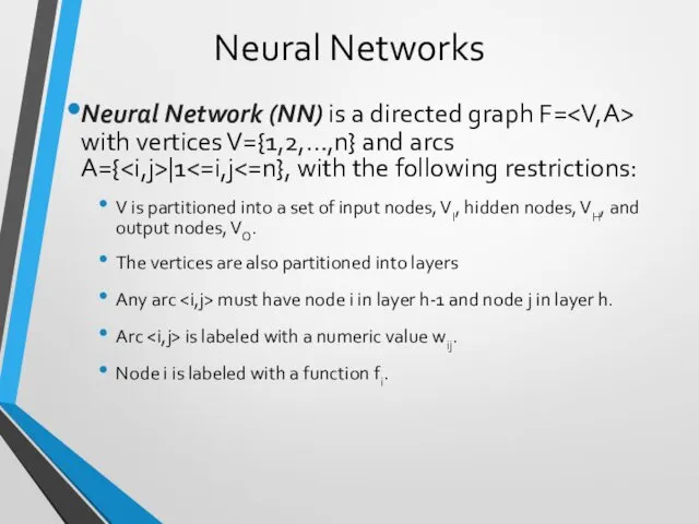
Neural Network (NN) is a directed graph F= with vertices
Neural Networks
Neural Network (NN) is a directed graph F=
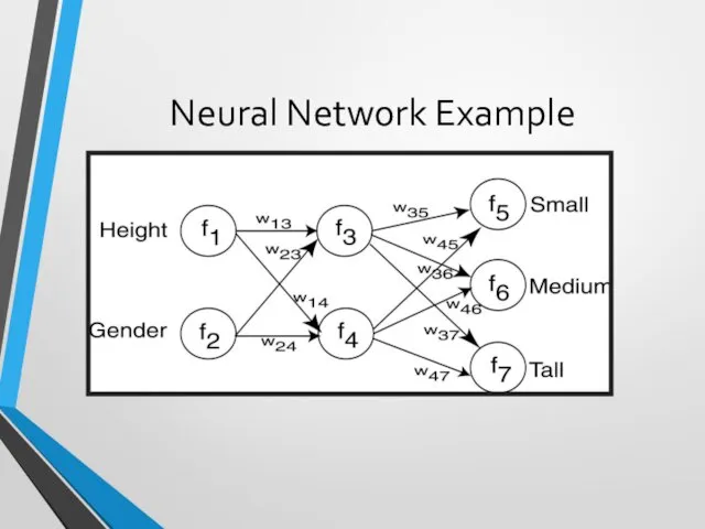
Neural Network Example
Neural Network Example
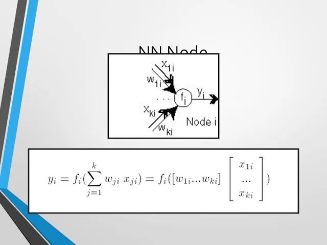
NN Node
NN Node
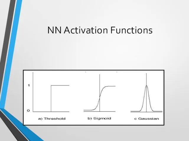
NN Activation Functions
Functions associated with nodes in graph.
Output may be in
NN Activation Functions
Functions associated with nodes in graph.
Output may be in
NN Activation Functions
NN Activation Functions
NN Learning
Propagate input values through graph.
Compare output to desired output.
Adjust weights
NN Learning
Propagate input values through graph.
Compare output to desired output.
Adjust weights
Neural Networks
A Neural Network Model is a computational model consisting of
Neural Networks
A Neural Network Model is a computational model consisting of
NN Advantages
Learning
Can continue learning even after training set has been applied.
Easy
NN Advantages
Learning
Can continue learning even after training set has been applied.
Easy
 Игровые технологии на уроках иностранного языка
 Городецкая роспись
 Виртуальная выставка Светлый образ матери
 Проект Путешествие капельки
 Рентгеноанатомия и методика рентгенологического исследования верхних отделов ЖКТ
 Задание В1. Тренажер
 Решение задач и выражений
 Джанни Родари Джельсомино в Стране Лжецов. Викторина
 20231112_prezentatsiya_fontan_gerona
 Параллелограмм. Виды параллелограммов и их свойства
 Автоматизация технологических процессов Курс лекций. Лекция 0. Введение
 Мастер-класс Пасхальный подарок
 Согласие да лад для общего дела клад
 Заветы Соодой-ламы
 Н.Гумилёв Слово
 6 класс: Движения земли
 Равнокрылые насекомые
 Защита программы лагеря
 Макет проекта Умник
 Разработка обобщающего урока на тему Жизнь на Земле, 5 класс
 Оптические процессоры
 Физминутка Веселые снеговики
 Электронные выпрямители. Классификация. Идеализация схем выпрямления
 Использование приемов мнемотехники в логопедической работе
 Обучение воспитанников с низким уровнем базовой подготовки по предмету (на примере учащихся школы воспитательной колонии).
 Obowiązywanie prawa. Termin ten jest wieloznaczny
 Проектирование зданий с использованием нетрадиционных источников энергии (биогаза)
 Вязание крючком ажурной салфетки. Второй тур олимпиады по технологии