- Public Economics

Содержание
- 2. Requirements 4+ homeworks Project Final exam Distribution: 40-20-40 read before class no cheating
- 3. Textbooks J. Gruber "Public Finance and Public Policy," Worth Publishers, 2007 or later editions Russian translation
- 4. Topics 1. Subject and methods of Public Finance. 2. Externalities. Applications to Environment and Health. 3.
- 5. Topics (cont) 6. Social Insurance. Adverse selection and moral hazard. 7. Social security. Unemployment insurance. 8.
- 6. Introduction What is the proper role of government? Expenditure side: What services should the government provide?
- 7. THE FOUR QUESTIONS OF PUBLIC FINANCE When should the government intervene in the economy? How might
- 8. When Should the Government Intervene in the Economy? Normally, private markets are competitive and efficient. Generally
- 9. When Should the Government Intervene? Market failures “Problems” for markets: Externalities Private (Asymmetric) Information Small number
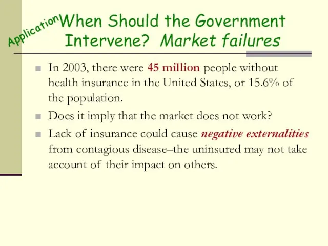
- 10. When Should the Government Intervene? Market failures In 2003, there were 45 million people without health
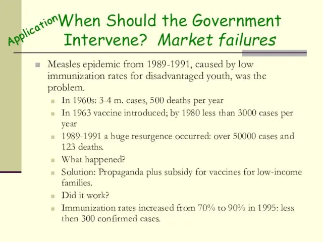
- 11. When Should the Government Intervene? Market failures Measles epidemic from 1989-1991, caused by low immunization rates
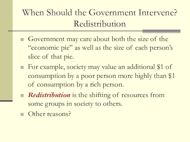
- 12. When Should the Government Intervene? Redistribution Government may care about both the size of the “economic
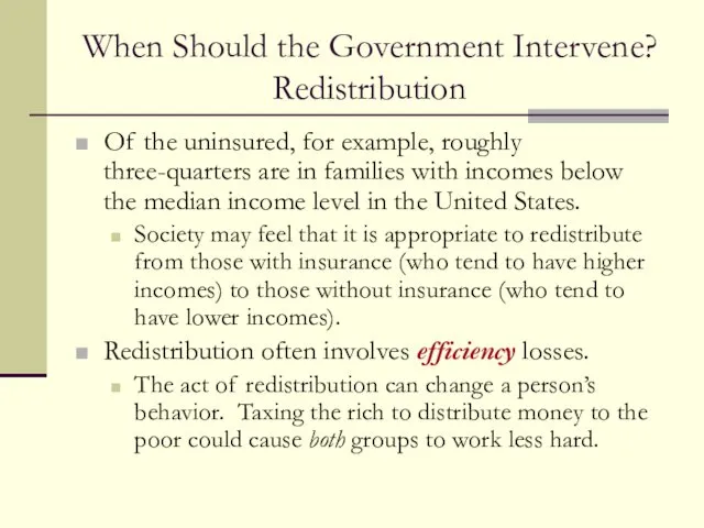
- 13. When Should the Government Intervene? Redistribution Of the uninsured, for example, roughly three-quarters are in families
- 14. How Might the Government Intervene? If the government wants to intervene in a market, there are
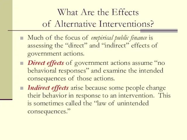
- 15. What Are the Effects of Alternative Interventions? Much of the focus of empirical public finance is
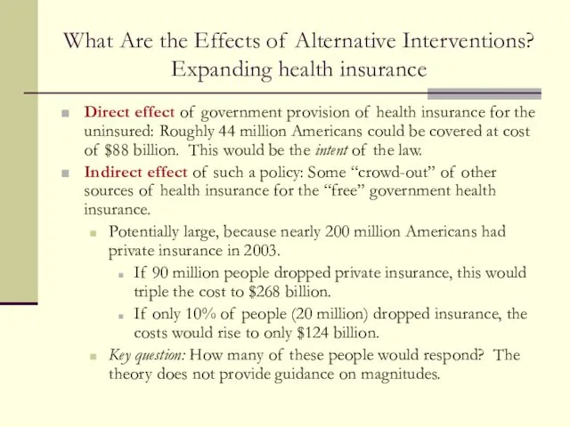
- 16. What Are the Effects of Alternative Interventions? Expanding health insurance Direct effect of government provision of
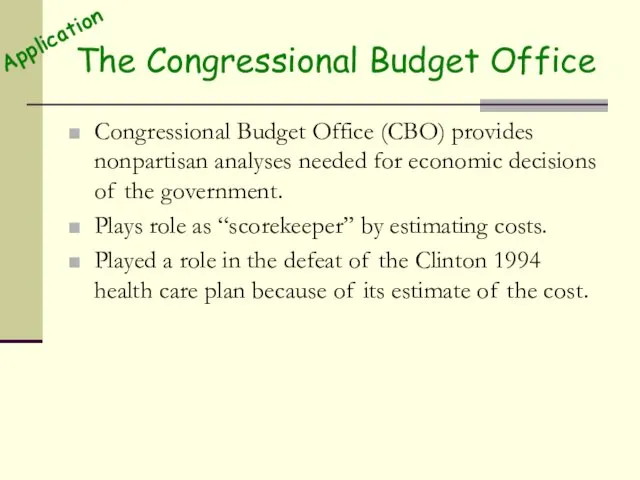
- 17. The Congressional Budget Office Congressional Budget Office (CBO) provides nonpartisan analyses needed for economic decisions of
- 18. Why Do Governments Do What They Do? Governments do not simply behave as benign actors who
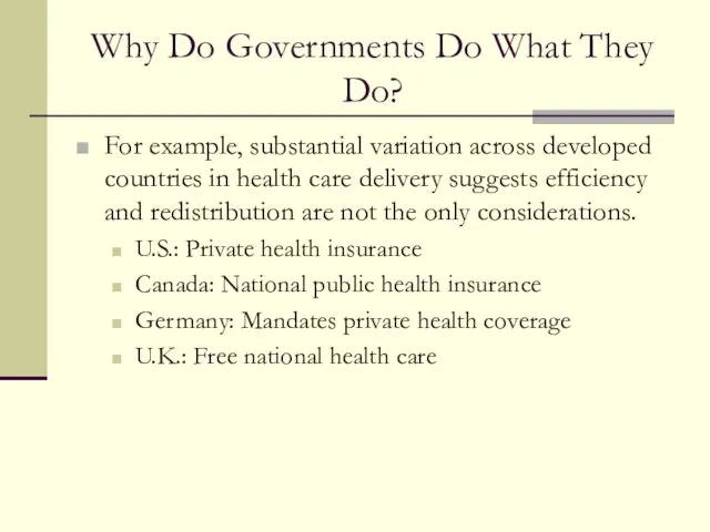
- 19. Why Do Governments Do What They Do? For example, substantial variation across developed countries in health
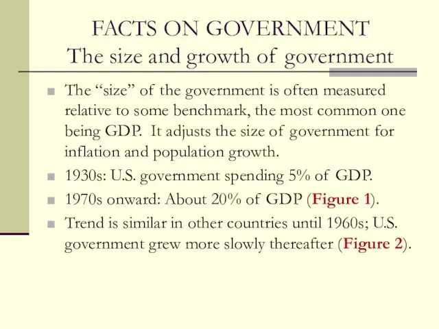
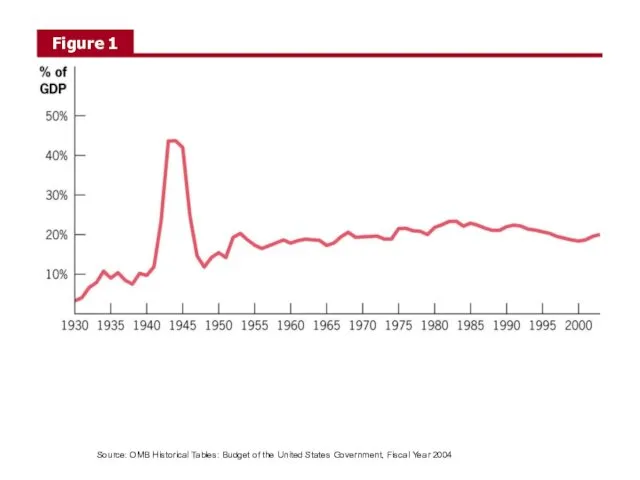
- 20. FACTS ON GOVERNMENT The size and growth of government The “size” of the government is often
- 21. Source: OMB Historical Tables: Budget of the United States Government, Fiscal Year 2004
- 22. Source: OECD Historical Statistics
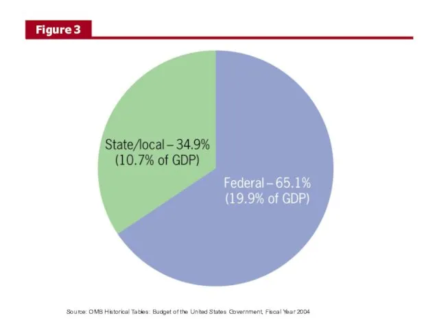
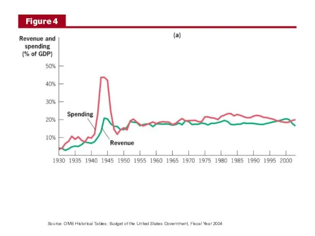
- 23. FACTS ON GOVERNMENT Decentralization and budgeting Other features Decentralization: In the United States., local, state and
- 24. Source: OMB Historical Tables: Budget of the United States Government, Fiscal Year 2004
- 25. Source: OMB Historical Tables: Budget of the United States Government, Fiscal Year 2004
- 26. FACTS ON GOVERNMENT Distribution of spending Other features Distribution of spending (Figure 7). In 1960: over
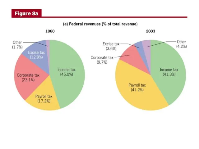
- 28. FACTS ON GOVERNMENT Distribution of revenue sources Other features Distribution of revenue (Figure 8a and 8b).
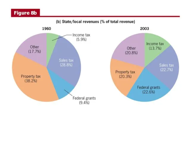
- 29. FACTS ON GOVERNMENT Distribution of revenue sources Other features Distribution of revenue different at state/local level.
- 32. FACTS ON GOVERNMENT Regulatory role of the government Other features Regulatory role–does not usually show up
- 33. Recap Four key questions in public finance When should the government intervene in the economy? How
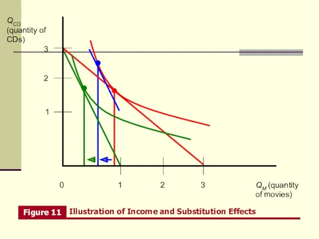
- 34. Theoretical tools (recap): Income and substitution effects. Equivalent and compensating variations. Consumer surplus. What are the
- 35. QM (quantity of movies) QCD (quantity of CDs) 0 1 2 1 2 3 3
- 36. Spectrum auctions: Governments sell licenses to use a certain range of frequencies (electromagnetic spectrum). Many auctions.
- 37. Dynamic Optimal taxation. (Acemoglu, Golosov, Tsyvinski)
- 38. PUTTING THE TOOLS TO WORK TANF and labor supply among single mothers TANF is “Temporary Assistance
- 39. PUTTING THE TOOLS TO WORK Identifying the budget constraint What does the budget constraint look like?
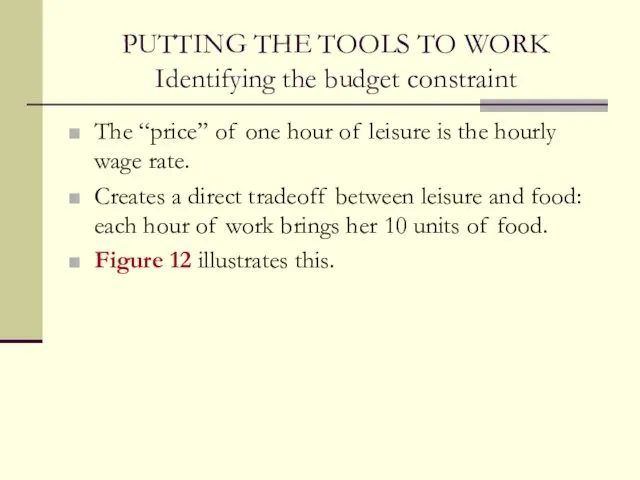
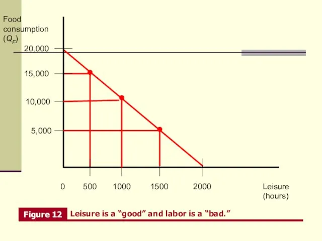
- 40. PUTTING THE TOOLS TO WORK Identifying the budget constraint The “price” of one hour of leisure
- 41. Leisure (hours) Food consumption (QF) 0 1000 1500 20,000 2000 500 15,000 10,000 5,000
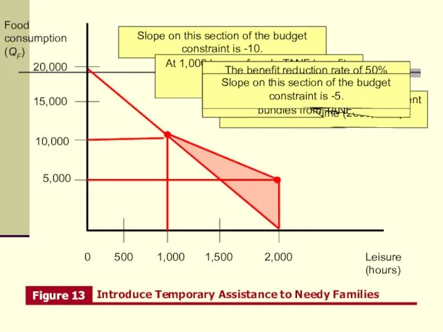
- 42. PUTTING THE TOOLS TO WORK The effect of TANF on the budget constraint Now, let’s introduce
- 43. PUTTING THE TOOLS TO WORK The effect of TANF on the budget constraint Assume that benefit
- 44. Leisure (hours) Food consumption (QF) 0 1,000 1,500 20,000 2,000 500 15,000 10,000 5,000 Slope on
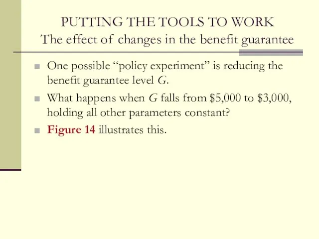
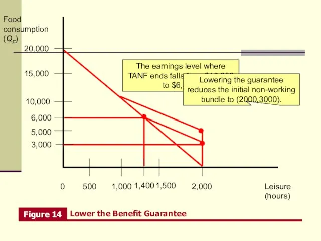
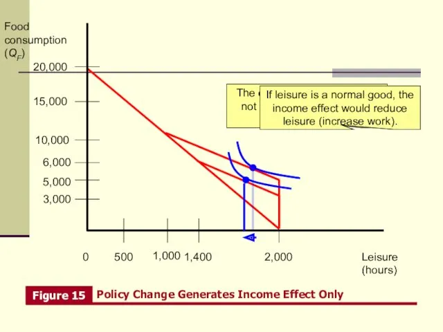
- 45. PUTTING THE TOOLS TO WORK The effect of changes in the benefit guarantee One possible “policy
- 46. Leisure (hours) Food consumption (QF) 0 1,000 1,500 20,000 2,000 500 15,000 10,000 5,000 3,000 1,400
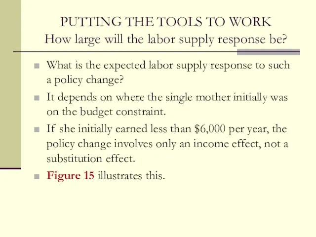
- 47. PUTTING THE TOOLS TO WORK How large will the labor supply response be? What is the
- 48. Leisure (hours) Food consumption (QF) 0 1,000 20,000 2,000 500 15,000 10,000 5,000 3,000 1,400 6,000
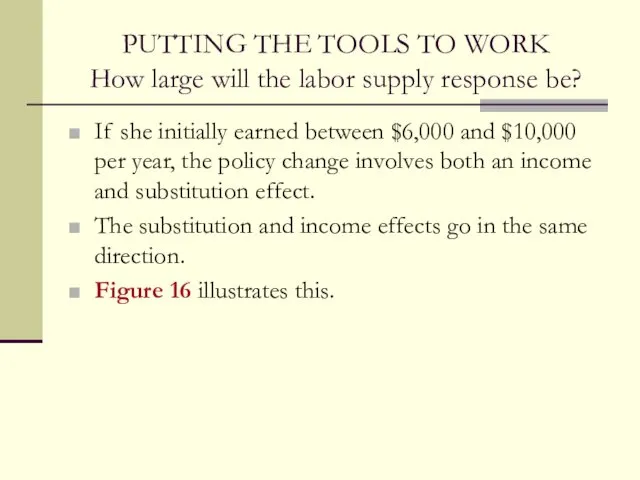
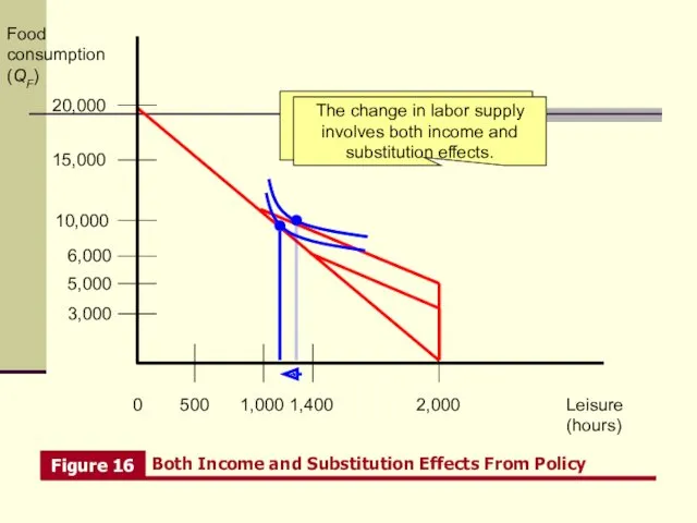
- 49. PUTTING THE TOOLS TO WORK How large will the labor supply response be? If she initially
- 50. Leisure (hours) Food consumption (QF) 0 1,000 20,000 2,000 500 15,000 10,000 5,000 3,000 1,400 6,000
- 51. PUTTING THE TOOLS TO WORK How large will the labor supply response be? Economic theory clearly
- 52. Leisure (hours) Food consumption (QF) 0 1,000 20,000 2,000 500 15,000 10,000 5,000 3,000 1,400 6,000
- 53. PUTTING THE TOOLS TO WORK How large will the labor supply response be? The actual magnitude
- 54. WELFARE IMPLICATIONS OF BENEFIT REDUCTIONS: TANF continued Efficiency and equity considerations in introducing or cutting TANF
- 55. Hours worked Wage H3 Labor demand w3 H2 w2 H1 w1 Labor supply Equilibrium with no
- 57. Скачать презентацию
Requirements
4+ homeworks
Project
Final exam
Distribution: 40-20-40
read before class
no cheating
Requirements
4+ homeworks
Project
Final exam
Distribution: 40-20-40
read before class
no cheating
Textbooks
J. Gruber "Public Finance and Public Policy," Worth Publishers, 2007
Textbooks
J. Gruber "Public Finance and Public Policy," Worth Publishers, 2007
Topics
1. Subject and methods of Public Finance.
2. Externalities. Applications to Environment
Topics
1. Subject and methods of Public Finance.
2. Externalities. Applications to Environment
Topics (cont)
6. Social Insurance. Adverse selection and moral hazard.
7. Social security.
Topics (cont)
6. Social Insurance. Adverse selection and moral hazard.
7. Social security.
Introduction
What is the proper role of government?
Expenditure side: What services should
Introduction
What is the proper role of government?
Expenditure side: What services should
THE FOUR QUESTIONS
OF PUBLIC FINANCE
When should the government intervene in
THE FOUR QUESTIONS
OF PUBLIC FINANCE
When should the government intervene in
When Should the Government Intervene in the Economy?
Normally, private markets are
When Should the Government Intervene in the Economy?
Normally, private markets are
When Should the Government Intervene? Market failures
“Problems” for markets:
Externalities
Private (Asymmetric) Information
Small
When Should the Government Intervene? Market failures
“Problems” for markets:
Externalities
Private (Asymmetric) Information
Small
When Should the Government Intervene? Market failures
In 2003, there were 45
When Should the Government Intervene? Market failures
In 2003, there were 45
When Should the Government Intervene? Market failures
Measles epidemic from 1989-1991, caused
When Should the Government Intervene? Market failures
Measles epidemic from 1989-1991, caused
When Should the Government Intervene?
Redistribution
Government may care about both the size
When Should the Government Intervene?
Redistribution
Government may care about both the size
When Should the Government Intervene?
Redistribution
Of the uninsured, for example, roughly three-quarters
When Should the Government Intervene?
Redistribution
Of the uninsured, for example, roughly three-quarters
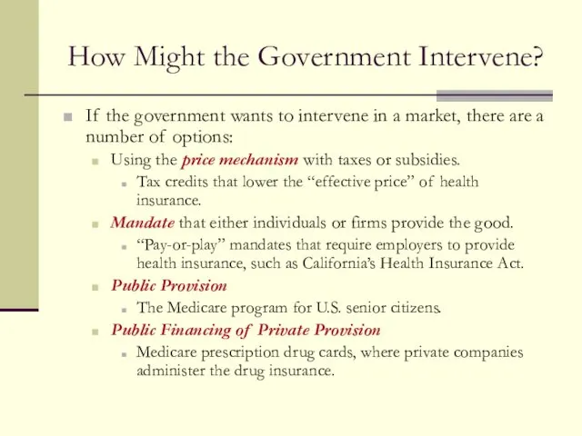
How Might the Government Intervene?
If the government wants to intervene in
How Might the Government Intervene?
If the government wants to intervene in
What Are the Effects
of Alternative Interventions?
Much of the focus of empirical
What Are the Effects
of Alternative Interventions?
Much of the focus of empirical
What Are the Effects of Alternative Interventions?
Expanding health insurance
Direct effect of
What Are the Effects of Alternative Interventions?
Expanding health insurance
Direct effect of
The Congressional Budget Office
Congressional Budget Office (CBO) provides nonpartisan analyses needed
The Congressional Budget Office
Congressional Budget Office (CBO) provides nonpartisan analyses needed
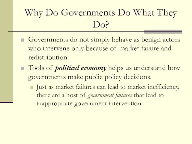
Why Do Governments Do What They Do?
Governments do not simply behave
Why Do Governments Do What They Do?
Governments do not simply behave
Why Do Governments Do What They Do?
For example, substantial variation across
Why Do Governments Do What They Do?
For example, substantial variation across
FACTS ON GOVERNMENT
The size and growth of government
The “size” of the
FACTS ON GOVERNMENT
The size and growth of government
The “size” of the
Source: OMB Historical Tables: Budget of the United States Government, Fiscal
Source: OMB Historical Tables: Budget of the United States Government, Fiscal
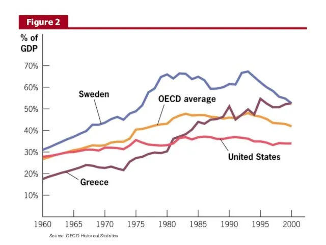
Source: OECD Historical Statistics
Source: OECD Historical Statistics
FACTS ON GOVERNMENT
Decentralization and budgeting
Other features
Decentralization: In the United States., local,
FACTS ON GOVERNMENT
Decentralization and budgeting
Other features
Decentralization: In the United States., local,
Source: OMB Historical Tables: Budget of the United States Government, Fiscal
Source: OMB Historical Tables: Budget of the United States Government, Fiscal
Source: OMB Historical Tables: Budget of the United States Government, Fiscal
Source: OMB Historical Tables: Budget of the United States Government, Fiscal
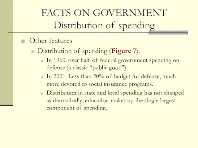
FACTS ON GOVERNMENT
Distribution of spending
Other features
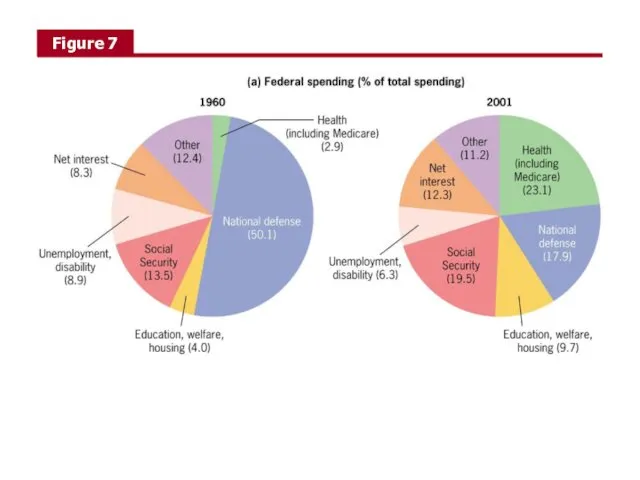
Distribution of spending (Figure 7).
In 1960:
FACTS ON GOVERNMENT
Distribution of spending
Other features
Distribution of spending (Figure 7).
In 1960:
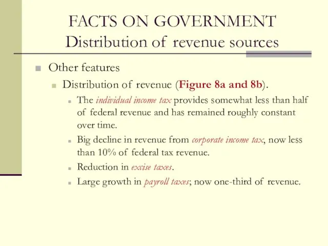
FACTS ON GOVERNMENT
Distribution of revenue sources
Other features
Distribution of revenue (Figure 8a
FACTS ON GOVERNMENT
Distribution of revenue sources
Other features
Distribution of revenue (Figure 8a
FACTS ON GOVERNMENT
Distribution of revenue sources
Other features
Distribution of revenue different at
FACTS ON GOVERNMENT
Distribution of revenue sources
Other features
Distribution of revenue different at

FACTS ON GOVERNMENT
Regulatory role of the government
Other features
Regulatory role–does not usually
FACTS ON GOVERNMENT
Regulatory role of the government
Other features
Regulatory role–does not usually
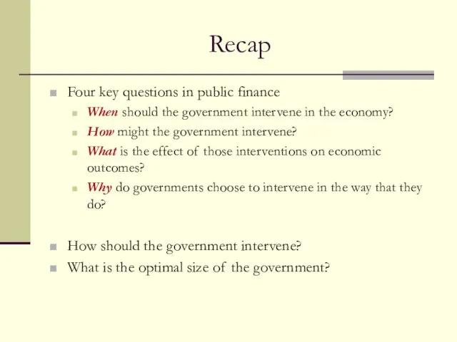
Recap
Four key questions in public finance
When should the government intervene in
Recap
Four key questions in public finance
When should the government intervene in
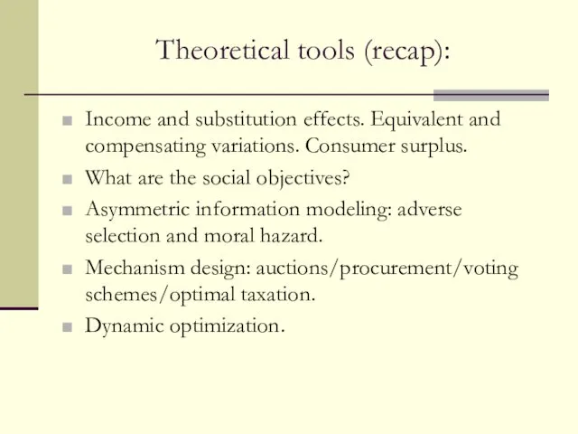
Theoretical tools (recap):
Income and substitution effects. Equivalent and compensating variations. Consumer
Theoretical tools (recap):
Income and substitution effects. Equivalent and compensating variations. Consumer
QM (quantity of movies)
QCD (quantity of CDs)
0
1
2
1
2
3
3
QM (quantity of movies)
QCD (quantity of CDs)
0
1
2
1
2
3
3

Spectrum auctions:
Governments sell licenses to use a certain range of frequencies
Spectrum auctions:
Governments sell licenses to use a certain range of frequencies
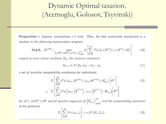
Dynamic Optimal taxation.
(Acemoglu, Golosov, Tsyvinski)
Dynamic Optimal taxation.
(Acemoglu, Golosov, Tsyvinski)
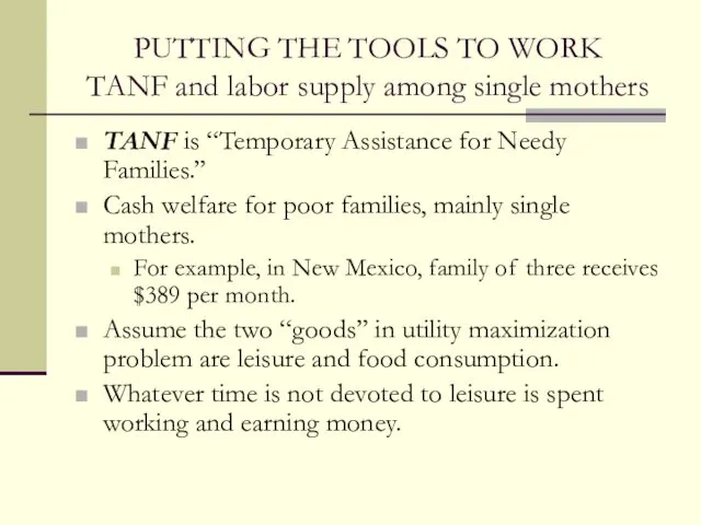
PUTTING THE TOOLS TO WORK
TANF and labor supply among single mothers
TANF
PUTTING THE TOOLS TO WORK
TANF and labor supply among single mothers
TANF
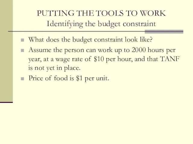
PUTTING THE TOOLS TO WORK
Identifying the budget constraint
What does the budget
PUTTING THE TOOLS TO WORK
Identifying the budget constraint
What does the budget
PUTTING THE TOOLS TO WORK
Identifying the budget constraint
The “price” of one
PUTTING THE TOOLS TO WORK
Identifying the budget constraint
The “price” of one
Leisure (hours)
Food consumption (QF)
0
1000
1500
20,000
2000
500
15,000
10,000
5,000
Leisure (hours)
Food consumption (QF)
0
1000
1500
20,000
2000
500
15,000
10,000
5,000
PUTTING THE TOOLS TO WORK
The effect of TANF on the budget
PUTTING THE TOOLS TO WORK The effect of TANF on the budget
PUTTING THE TOOLS TO WORK
The effect of TANF on the budget
PUTTING THE TOOLS TO WORK The effect of TANF on the budget
Leisure (hours)
Food consumption (QF)
0
1,000
1,500
20,000
2,000
500
15,000
10,000
5,000
Slope on this section of the budget constraint
Leisure (hours)
Food consumption (QF)
0
1,000
1,500
20,000
2,000
500
15,000
10,000
5,000
Slope on this section of the budget constraint
PUTTING THE TOOLS TO WORK
The effect of changes in the benefit
PUTTING THE TOOLS TO WORK The effect of changes in the benefit
Leisure (hours)
Food consumption (QF)
0
1,000
1,500
20,000
2,000
500
15,000
10,000
5,000
3,000
1,400
6,000
The earnings level where TANF ends falls from
Leisure (hours)
Food consumption (QF)
0
1,000
1,500
20,000
2,000
500
15,000
10,000
5,000
3,000
1,400
6,000
The earnings level where TANF ends falls from
PUTTING THE TOOLS TO WORK
How large will the labor supply response
PUTTING THE TOOLS TO WORK How large will the labor supply response
Leisure (hours)
Food consumption (QF)
0
1,000
20,000
2,000
500
15,000
10,000
5,000
3,000
1,400
6,000
The effective wage rate does not change for
Leisure (hours)
Food consumption (QF)
0
1,000
20,000
2,000
500
15,000
10,000
5,000
3,000
1,400
6,000
The effective wage rate does not change for
PUTTING THE TOOLS TO WORK
How large will the labor supply response
PUTTING THE TOOLS TO WORK How large will the labor supply response
Leisure (hours)
Food consumption (QF)
0
1,000
20,000
2,000
500
15,000
10,000
5,000
3,000
1,400
6,000
The effective wage rate changes for this person.
The
Leisure (hours)
Food consumption (QF)
0
1,000
20,000
2,000
500
15,000
10,000
5,000
3,000
1,400
6,000
The effective wage rate changes for this person.
The
PUTTING THE TOOLS TO WORK
How large will the labor supply response
PUTTING THE TOOLS TO WORK How large will the labor supply response
Leisure (hours)
Food consumption (QF)
0
1,000
20,000
2,000
500
15,000
10,000
5,000
3,000
1,400
6,000
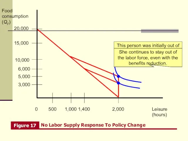
This person was initially out of the labor
Leisure (hours)
Food consumption (QF)
0
1,000
20,000
2,000
500
15,000
10,000
5,000
3,000
1,400
6,000
This person was initially out of the labor

PUTTING THE TOOLS TO WORK
How large will the labor supply response
PUTTING THE TOOLS TO WORK How large will the labor supply response
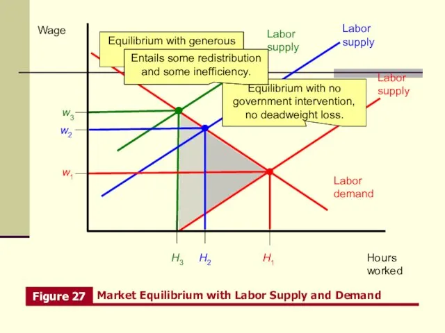
WELFARE IMPLICATIONS OF BENEFIT REDUCTIONS: TANF continued
Efficiency and equity considerations in
WELFARE IMPLICATIONS OF BENEFIT REDUCTIONS: TANF continued
Efficiency and equity considerations in
Hours worked
Wage
H3
Labor demand
w3
H2
w2
H1
w1
Labor supply
Equilibrium with no government intervention, no deadweight loss.
Labor
Hours worked
Wage
H3
Labor demand
w3
H2
w2
H1
w1
Labor supply
Equilibrium with no government intervention, no deadweight loss.
Labor
 Самоиндукция. Индуктивность
 Частотно – регулируемый асинхронный электропривод
 Правотворчество и формирование закона
 Деревянные балки в покрытиях и перекрытиях
 Сердечнолегочная реанимация у детей
 Конкурентные преимущества Raw Life Protein
 Роль родного языка и речи в развитии ребенка
 НУЗ Дорожная клиническая больница ОАО РЖД. Преимущества на рынке медицинских услуг
 Организация контроля на уроках информатики
 Approaches. Discussion
 Таблица умножения и деления на 2
 Импульс тела. Закон сохранения импульса. Реактивное движение
 Право на образование
 Старая Уфа
 Доказательная медицина. Формулярная система. Фармакоэпидемиология
 Казань - спортивная столица
 Социальное партнёрство с родителями, как условие развития творческих способностей обучающихся
  Разработка GIF-анимации через Photoshop
 Основні симптоми та синдроми при цукровому діабеті
 Неопределенные местоимения
 Системы двух линейных уравнений с двумя переменными, как математические модели реальных ситуаций. 7 класс
 Колядки
 Грыжи. Классификация грыж
 Методы исследования механической активности сердца
 Производство облицовочных работ
 Ресторан BigMama
 Психические и поведенческие расстройства в результате употребления летучих растворителей (ингалянтов)
 Презентация проекта Волшебная пуговица.