- Basics of factor models

Содержание
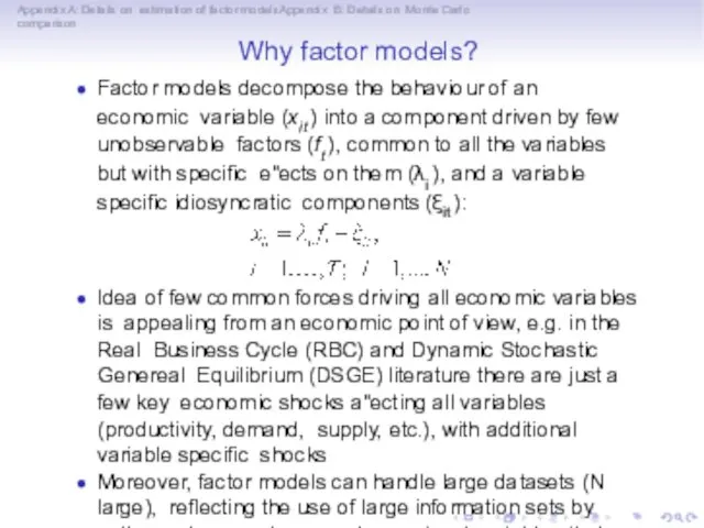
- 2. Appendix A: Details on estimation of factor modelsAppendix B: Details on Monte Carlo comparison Why factor
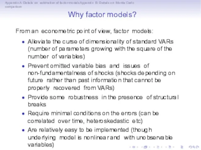
- 3. Appendix A: Details on estimation of factor modelsAppendix B: Details on Monte Carlo comparison Why factor
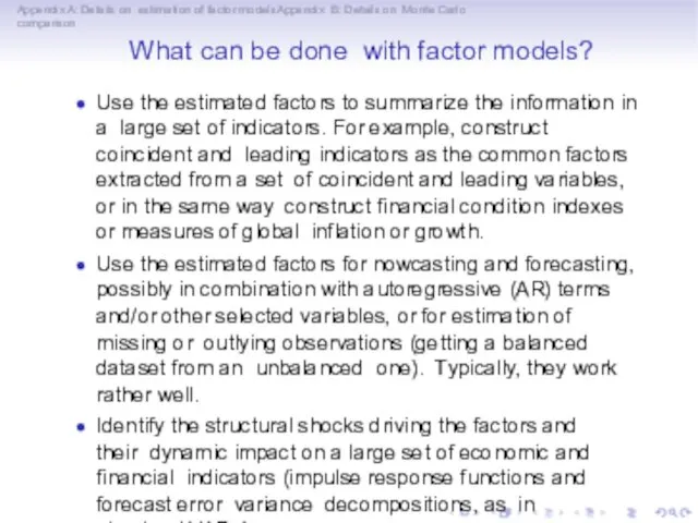
- 4. Appendix A: Details on estimation of factor modelsAppendix B: Details on Monte Carlo comparison What can
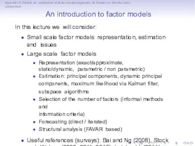
- 5. Appendix A: Details on estimation of factor modelsAppendix B: Details on Monte Carlo comparison An introduction
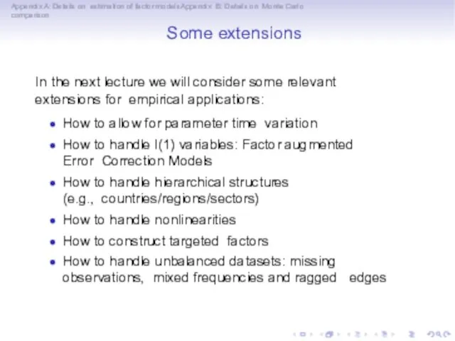
- 6. Appendix A: Details on estimation of factor modelsAppendix B: Details on Monte Carlo comparison Some extensions
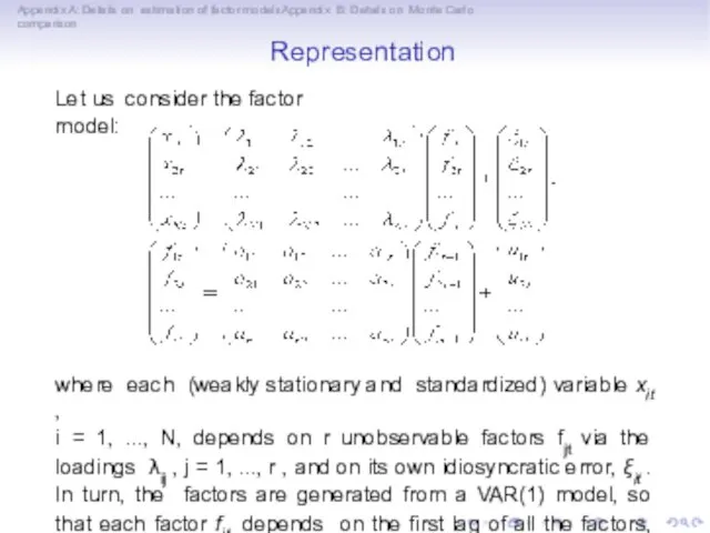
- 7. Appendix A: Details on estimation of factor modelsAppendix B: Details on Monte Carlo comparison Representation Let
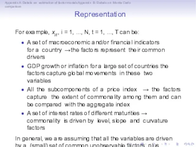
- 8. Appendix A: Details on estimation of factor modelsAppendix B: Details on Monte Carlo comparison Representation For
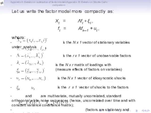
- 9. Appendix A: Details on estimation of factor modelsAppendix B: Details on Monte Carlo comparison Let us
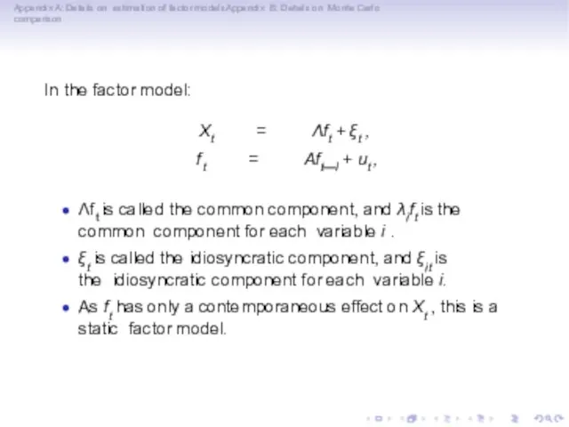
- 10. Appendix A: Details on estimation of factor modelsAppendix B: Details on Monte Carlo comparison In the
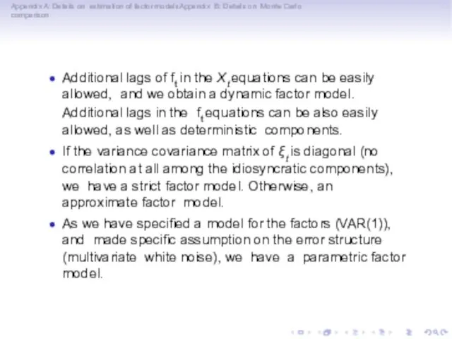
- 11. Appendix A: Details on estimation of factor modelsAppendix B: Details on Monte Carlo comparison Additional lags
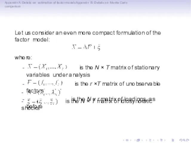
- 12. Appendix A: Details on estimation of factor modelsAppendix B: Details on Monte Carlo comparison Let us
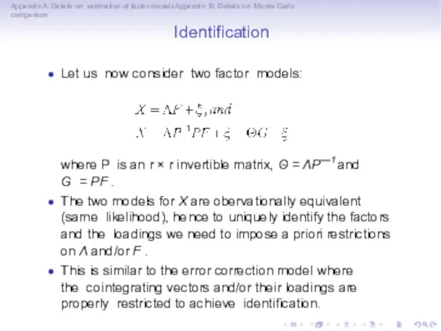
- 13. Appendix A: Details on estimation of factor modelsAppendix B: Details on Monte Carlo comparison Identification Let
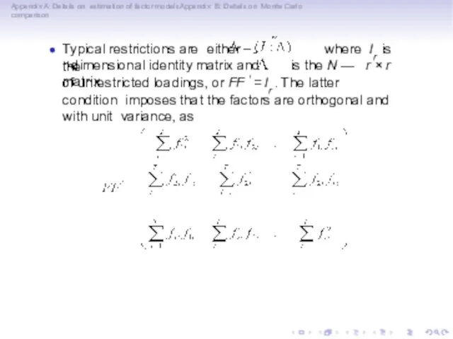
- 14. Appendix A: Details on estimation of factor modelsAppendix B: Details on Monte Carlo comparison Typical restrictions
- 15. Appendix A: Details on estimation of factor modelsAppendix B: Details on Monte Carlo comparison The condition
- 16. Appendix A: Details on estimation of factor modelsAppendix B: Details on Monte Carlo comparison Factor models
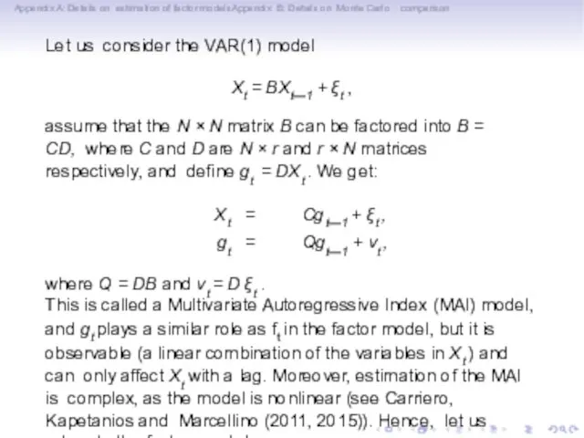
- 17. Appendix A: Details on estimation of factor modelsAppendix B: Details on Monte Carlo comparison Let us
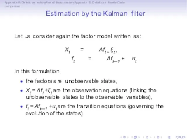
- 18. Appendix A: Details on estimation of factor modelsAppendix B: Details on Monte Carlo comparison Estimation by
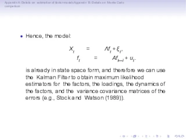
- 19. Appendix A: Details on estimation of factor modelsAppendix B: Details on Monte Carlo comparison Hence, the
- 20. Appendix A: Details on estimation of factor modelsAppendix B: Details on Monte Carlo comparison However, there
- 21. Appendix A: Details on estimation of factor modelsAppendix B: Details on Monte Carlo comparison Non-parametric, large
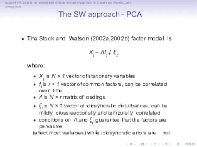
- 22. Appendix A: Details on estimation of factor modelsAppendix B: Details on Monte Carlo comparison The SW
- 23. Appendix A: Details on estimation of factor modelsAppendix B: Details on Monte Carlo comparison The SW
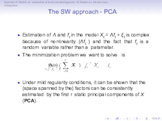
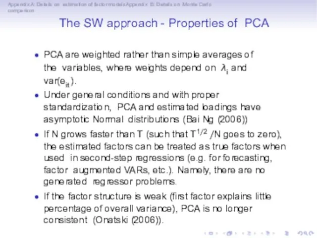
- 24. Appendix A: Details on estimation of factor modelsAppendix B: Details on Monte Carlo comparison The SW
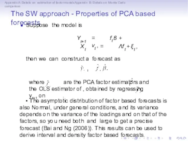
- 25. Appendix A: Details on estimation of factor modelsAppendix B: Details on Monte Carlo comparison The SW
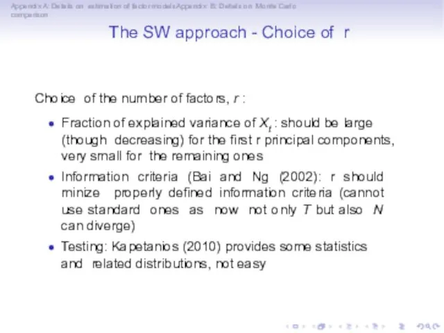
- 26. Appendix A: Details on estimation of factor modelsAppendix B: Details on Monte Carlo comparison The SW
- 27. Appendix A: Details on estimation of factor modelsAppendix B: Details on Monte Carlo comparison The SW
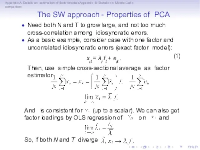
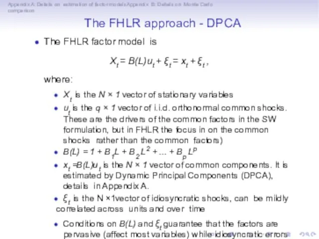
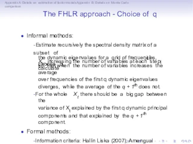
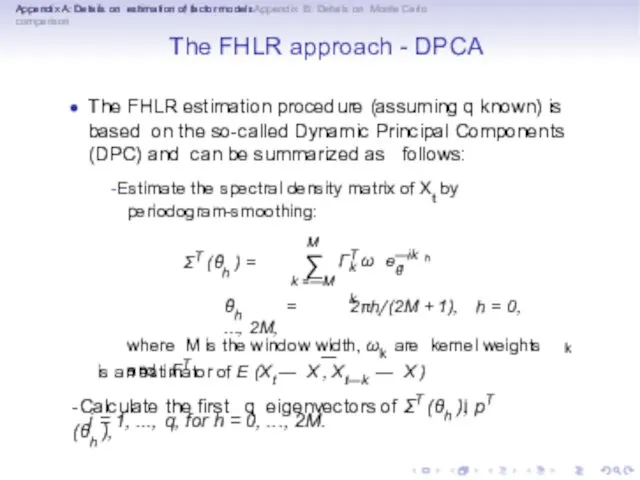
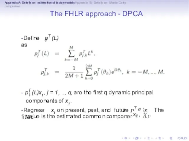
- 28. Appendix A: Details on estimation of factor modelsAppendix B: Details on Monte Carlo comparison The FHLR
- 29. Appendix A: Details on estimation of factor modelsAppendix B: Details on Monte Carlo comparison The FHLR
- 30. Appendix A: Details on estimation of factor modelsAppendix B: Details on Monte Carlo comparison The FHLR
- 31. Appendix A: Details on estimation of factor modelsAppendix B: Details on Monte Carlo comparison The FHLR
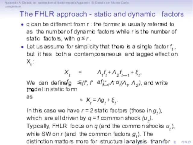
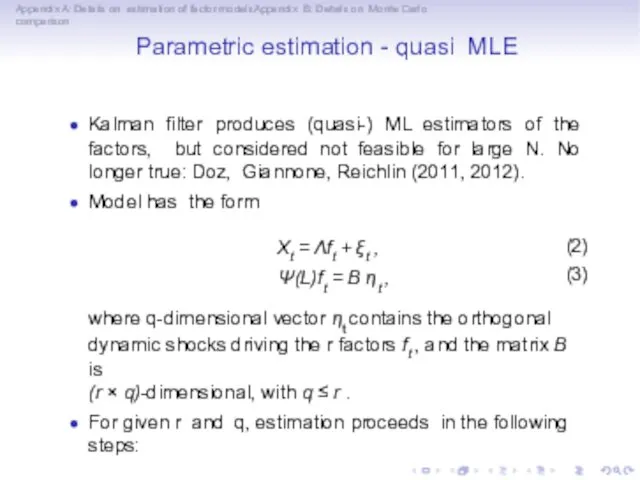
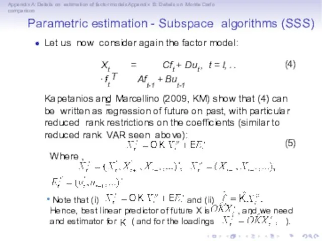
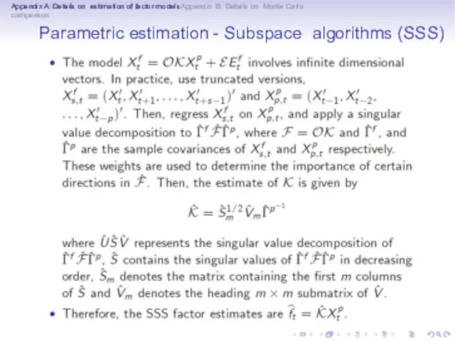
- 32. Appendix A: Details on estimation of factor modelsAppendix B: Details on Monte Carlo comparison Parametric estimation
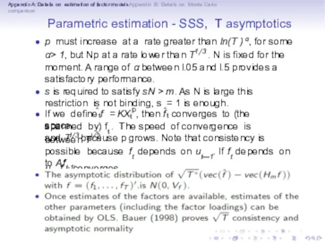
- 33. Appendix A: Details on estimation of factor modelsAppendix B: Details on Monte Carlo comparison Parametric estimation
- 34. Appendix A: Details on estimation of factor modelsAppendix B: Details on Monte Carlo comparison Parametric estimation
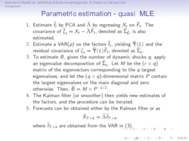
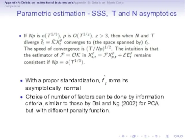
- 35. Appendix A: Details on estimation of factor modelsAppendix B: Details on Monte Carlo comparison Parametric estimation
- 36. Appendix A: Details on estimation of factor modelsAppendix B: Details on Monte Carlo comparison Parametric estimation
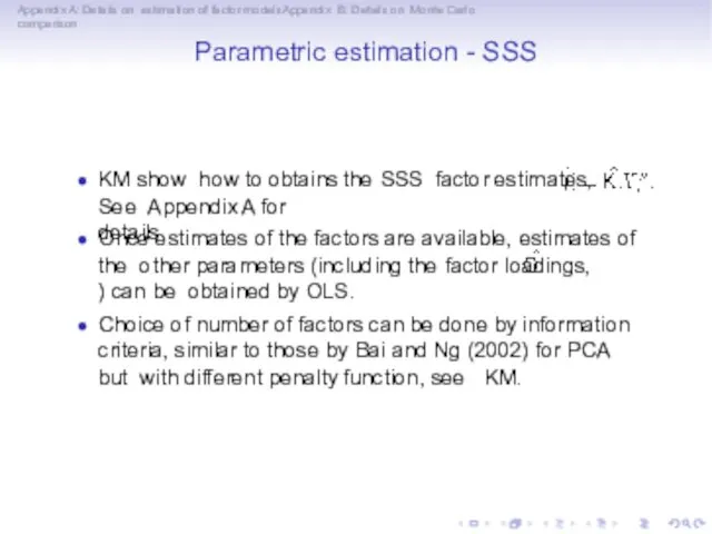
- 37. Appendix A: Details on estimation of factor modelsAppendix B: Details on Monte Carlo comparison Factor estimation
- 38. Appendix A: Details on estimation of factor modelsAppendix B: Details on Monte Carlo comparison Factor estimation
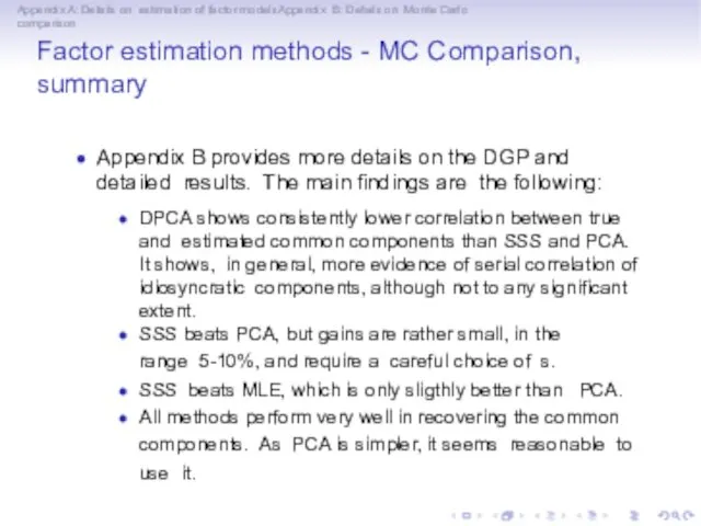
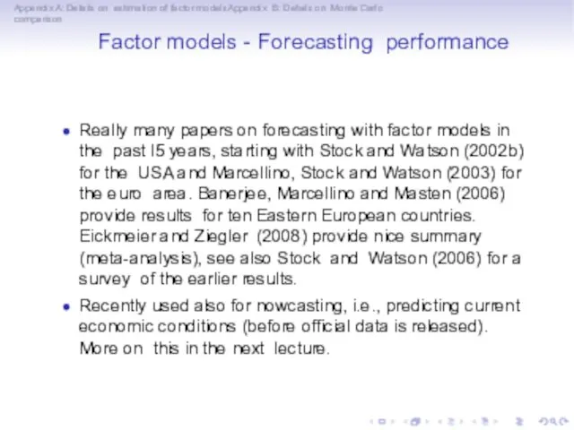
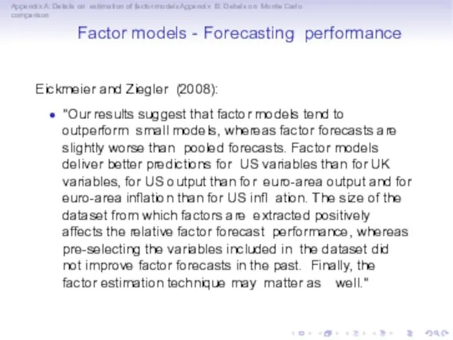
- 39. Appendix A: Details on estimation of factor modelsAppendix B: Details on Monte Carlo comparison Factor models
- 40. Appendix A: Details on estimation of factor modelsAppendix B: Details on Monte Carlo comparison Factor models
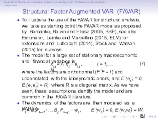
- 41. Appendix A: Details on estimation of factor modelsAppendix B: Details on Monte Carlo comparison Structural Factor
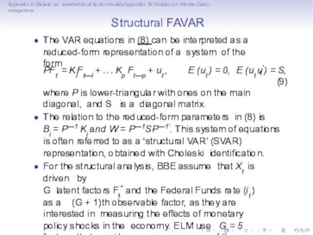
- 42. Appendix A: Details on estimation of factor modelsAppendix B: Details on Monte Carlo comparison Structural FAVAR
- 43. Appendix A: Details on estimation of factor modelsAppendix B: Details on Monte Carlo comparison Structural FAVAR
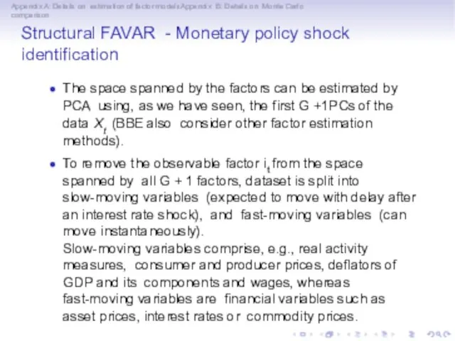
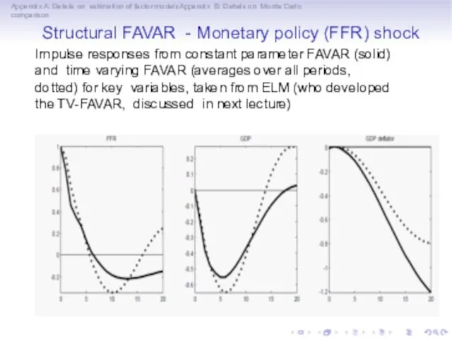
- 44. Appendix A: Details on estimation of factor modelsAppendix B: Details on Monte Carlo comparison Structural FAVAR
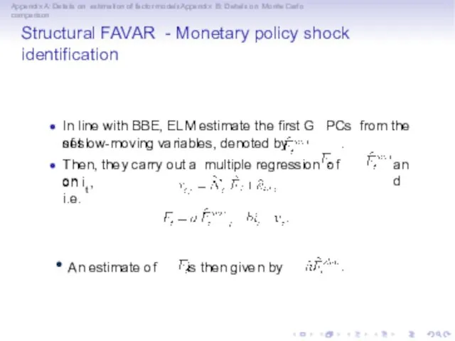
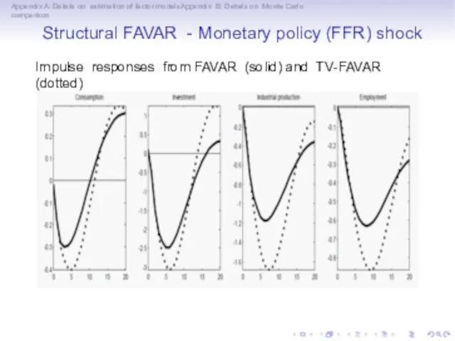
- 45. Appendix A: Details on estimation of factor modelsAppendix B: Details on Monte Carlo comparison Structural FAVAR
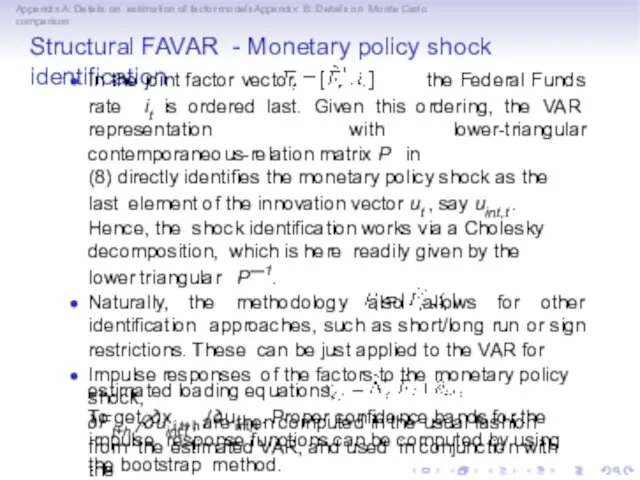
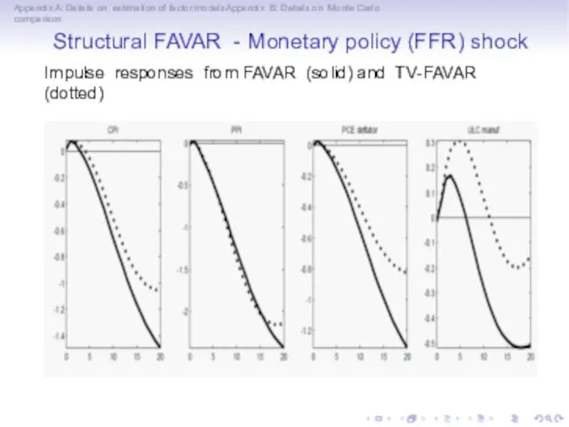
- 46. Appendix A: Details on estimation of factor modelsAppendix B: Details on Monte Carlo comparison Structural FAVAR
- 47. Appendix A: Details on estimation of factor modelsAppendix B: Details on Monte Carlo comparison Structural FAVAR
- 48. Appendix A: Details on estimation of factor modelsAppendix B: Details on Monte Carlo comparison Structural FAVAR
- 49. Appendix A: Details on estimation of factor modelsAppendix B: Details on Monte Carlo comparison Structural FAVAR:
- 50. Appendix A: Details on estimation of factor modelsAppendix B: Details on Monte Carlo comparison References Amengual,
- 51. Appendix A: Details on estimation of factor modelsAppendix B: Details on Monte Carlo comparison Banerjee, A.,
- 52. Appendix A: Details on estimation of factor modelsAppendix B: Details on Monte Carlo comparison Doz, C.,
- 53. Appendix A: Details on estimation of factor modelsAppendix B: Details on Monte Carlo comparison Forni, M.,
- 54. Appendix A: Details on estimation of factor modelsAppendix B: Details on Monte Carlo comparison Lutkepohl, H.
- 55. Appendix A: Details on estimation of factor modelsAppendix B: Details on Monte Carlo comparison Stock, J.H
- 56. Appendix A: Details on estimation of factor modelsAppendix B: Details on Monte Carlo comparison Stock, J.H.
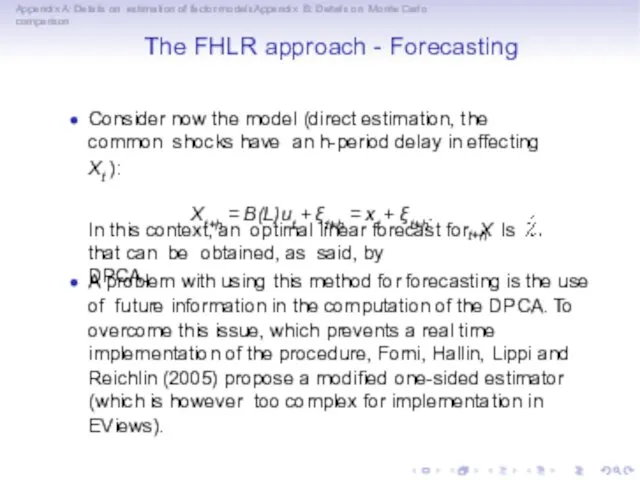
- 57. Appendix A: Details on estimation of factor modelsAppendix B: Details on Monte Carlo comparison The FHLR
- 58. Appendix A: Details on estimation of factor modelsAppendix B: Details on Monte Carlo comparison The FHLR
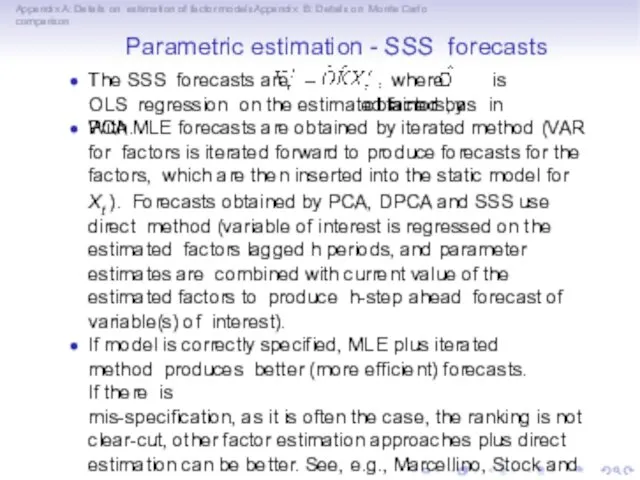
- 59. Appendix A: Details on estimation of factor modelsAppendix B: Details on Monte Carlo comparison Parametric estimation
- 60. Appendix A: Details on estimation of factor modelsAppendix B: Details on Monte Carlo comparison Parametric estimation
- 61. Appendix A: Details on estimation of factor modelsAppendix B: Details on Monte Carlo comparison Parametric estimation
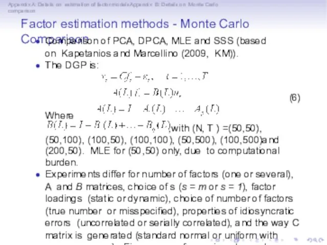
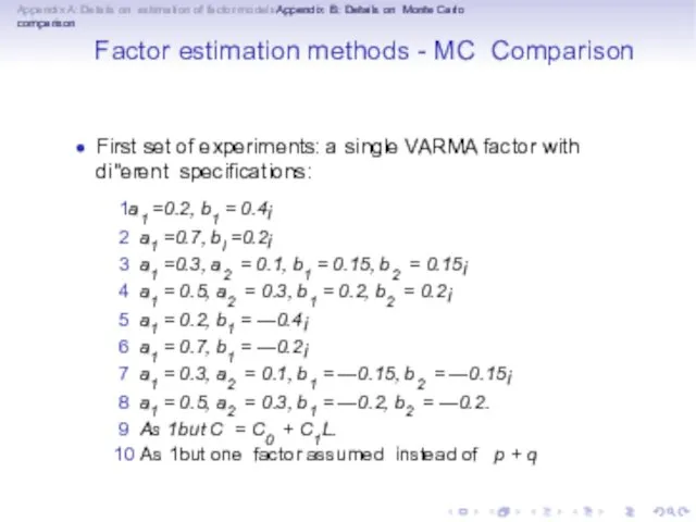
- 62. Appendix A: Details on estimation of factor modelsAppendix B: Details on Monte Carlo comparison Factor estimation
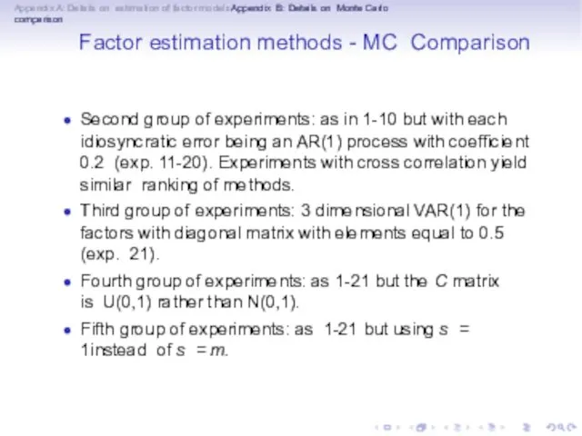
- 63. Appendix A: Details on estimation of factor modelsAppendix B: Details on Monte Carlo comparison Factor estimation
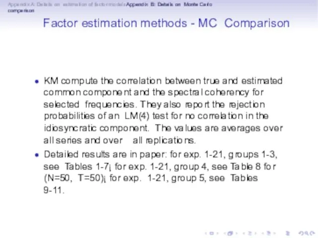
- 64. Appendix A: Details on estimation of factor modelsAppendix B: Details on Monte Carlo comparison Factor estimation
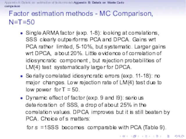
- 65. Appendix A: Details on estimation of factor modelsAppendix B: Details on Monte Carlo comparison Factor estimation
- 66. Appendix A: Details on estimation of factor modelsAppendix B: Details on Monte Carlo comparison Factor estimation
- 68. Скачать презентацию
Appendix A: Details on estimation of factor modelsAppendix B: Details on
Appendix A: Details on estimation of factor modelsAppendix B: Details on
Appendix A: Details on estimation of factor modelsAppendix B: Details on
Appendix A: Details on estimation of factor modelsAppendix B: Details on
Appendix A: Details on estimation of factor modelsAppendix B: Details on
Appendix A: Details on estimation of factor modelsAppendix B: Details on
Appendix A: Details on estimation of factor modelsAppendix B: Details on
Appendix A: Details on estimation of factor modelsAppendix B: Details on
Appendix A: Details on estimation of factor modelsAppendix B: Details on
Appendix A: Details on estimation of factor modelsAppendix B: Details on
Appendix A: Details on estimation of factor modelsAppendix B: Details on
Appendix A: Details on estimation of factor modelsAppendix B: Details on
Appendix A: Details on estimation of factor modelsAppendix B: Details on
Appendix A: Details on estimation of factor modelsAppendix B: Details on
Appendix A: Details on estimation of factor modelsAppendix B: Details on
Appendix A: Details on estimation of factor modelsAppendix B: Details on
Appendix A: Details on estimation of factor modelsAppendix B: Details on
Appendix A: Details on estimation of factor modelsAppendix B: Details on
Appendix A: Details on estimation of factor modelsAppendix B: Details on
Appendix A: Details on estimation of factor modelsAppendix B: Details on
Appendix A: Details on estimation of factor modelsAppendix B: Details on
Appendix A: Details on estimation of factor modelsAppendix B: Details on
Appendix A: Details on estimation of factor modelsAppendix B: Details on
Appendix A: Details on estimation of factor modelsAppendix B: Details on
Appendix A: Details on estimation of factor modelsAppendix B: Details on
Appendix A: Details on estimation of factor modelsAppendix B: Details on
Appendix A: Details on estimation of factor modelsAppendix B: Details on
Appendix A: Details on estimation of factor modelsAppendix B: Details on
Appendix A: Details on estimation of factor modelsAppendix B: Details on
Appendix A: Details on estimation of factor modelsAppendix B: Details on
Appendix A: Details on estimation of factor modelsAppendix B: Details on
Appendix A: Details on estimation of factor modelsAppendix B: Details on
Appendix A: Details on estimation of factor modelsAppendix B: Details on
Appendix A: Details on estimation of factor modelsAppendix B: Details on
Appendix A: Details on estimation of factor modelsAppendix B: Details on
Appendix A: Details on estimation of factor modelsAppendix B: Details on
Appendix A: Details on estimation of factor modelsAppendix B: Details on
Appendix A: Details on estimation of factor modelsAppendix B: Details on
Appendix A: Details on estimation of factor modelsAppendix B: Details on
Appendix A: Details on estimation of factor modelsAppendix B: Details on
Appendix A: Details on estimation of factor modelsAppendix B: Details on
Appendix A: Details on estimation of factor modelsAppendix B: Details on
Appendix A: Details on estimation of factor modelsAppendix B: Details on
Appendix A: Details on estimation of factor modelsAppendix B: Details on
Appendix A: Details on estimation of factor modelsAppendix B: Details on
Appendix A: Details on estimation of factor modelsAppendix B: Details on
Appendix A: Details on estimation of factor modelsAppendix B: Details on
Appendix A: Details on estimation of factor modelsAppendix B: Details on
Appendix A: Details on estimation of factor modelsAppendix B: Details on
Appendix A: Details on estimation of factor modelsAppendix B: Details on
Appendix A: Details on estimation of factor modelsAppendix B: Details on
Appendix A: Details on estimation of factor modelsAppendix B: Details on
Appendix A: Details on estimation of factor modelsAppendix B: Details on
Appendix A: Details on estimation of factor modelsAppendix B: Details on
Appendix A: Details on estimation of factor modelsAppendix B: Details on
Appendix A: Details on estimation of factor modelsAppendix B: Details on
Appendix A: Details on estimation of factor modelsAppendix B: Details on
Appendix A: Details on estimation of factor modelsAppendix B: Details on
Appendix A: Details on estimation of factor modelsAppendix B: Details on
Appendix A: Details on estimation of factor modelsAppendix B: Details on
Appendix A: Details on estimation of factor modelsAppendix B: Details on
Appendix A: Details on estimation of factor modelsAppendix B: Details on
Appendix A: Details on estimation of factor modelsAppendix B: Details on
Appendix A: Details on estimation of factor modelsAppendix B: Details on
Appendix A: Details on estimation of factor modelsAppendix B: Details on
Appendix A: Details on estimation of factor modelsAppendix B: Details on
Appendix A: Details on estimation of factor modelsAppendix B: Details on
Appendix A: Details on estimation of factor modelsAppendix B: Details on
Appendix A: Details on estimation of factor modelsAppendix B: Details on
Appendix A: Details on estimation of factor modelsAppendix B: Details on
Appendix A: Details on estimation of factor modelsAppendix B: Details on
Appendix A: Details on estimation of factor modelsAppendix B: Details on
Appendix A: Details on estimation of factor modelsAppendix B: Details on
Appendix A: Details on estimation of factor modelsAppendix B: Details on
Appendix A: Details on estimation of factor modelsAppendix B: Details on
Appendix A: Details on estimation of factor modelsAppendix B: Details on
Appendix A: Details on estimation of factor modelsAppendix B: Details on
Appendix A: Details on estimation of factor modelsAppendix B: Details on
Appendix A: Details on estimation of factor modelsAppendix B: Details on
Appendix A: Details on estimation of factor modelsAppendix B: Details on
Appendix A: Details on estimation of factor modelsAppendix B: Details on
Appendix A: Details on estimation of factor modelsAppendix B: Details on
Appendix A: Details on estimation of factor modelsAppendix B: Details on
Appendix A: Details on estimation of factor modelsAppendix B: Details on
Appendix A: Details on estimation of factor modelsAppendix B: Details on
Appendix A: Details on estimation of factor modelsAppendix B: Details on
Appendix A: Details on estimation of factor modelsAppendix B: Details on
Appendix A: Details on estimation of factor modelsAppendix B: Details on
Appendix A: Details on estimation of factor modelsAppendix B: Details on
Appendix A: Details on estimation of factor modelsAppendix B: Details on
Appendix A: Details on estimation of factor modelsAppendix B: Details on
Appendix A: Details on estimation of factor modelsAppendix B: Details on
Appendix A: Details on estimation of factor modelsAppendix B: Details on
Appendix A: Details on estimation of factor modelsAppendix B: Details on
Appendix A: Details on estimation of factor modelsAppendix B: Details on
Appendix A: Details on estimation of factor modelsAppendix B: Details on
Appendix A: Details on estimation of factor modelsAppendix B: Details on
Appendix A: Details on estimation of factor modelsAppendix B: Details on
Appendix A: Details on estimation of factor modelsAppendix B: Details on
Appendix A: Details on estimation of factor modelsAppendix B: Details on
Appendix A: Details on estimation of factor modelsAppendix B: Details on
Appendix A: Details on estimation of factor modelsAppendix B: Details on
Appendix A: Details on estimation of factor modelsAppendix B: Details on
Appendix A: Details on estimation of factor modelsAppendix B: Details on
Appendix A: Details on estimation of factor modelsAppendix B: Details on
Appendix A: Details on estimation of factor modelsAppendix B: Details on
Appendix A: Details on estimation of factor modelsAppendix B: Details on
Appendix A: Details on estimation of factor modelsAppendix B: Details on
Appendix A: Details on estimation of factor modelsAppendix B: Details on
Appendix A: Details on estimation of factor modelsAppendix B: Details on
Appendix A: Details on estimation of factor modelsAppendix B: Details on
Appendix A: Details on estimation of factor modelsAppendix B: Details on
Appendix A: Details on estimation of factor modelsAppendix B: Details on
Appendix A: Details on estimation of factor modelsAppendix B: Details on
Appendix A: Details on estimation of factor modelsAppendix B: Details on
Appendix A: Details on estimation of factor modelsAppendix B: Details on
Appendix A: Details on estimation of factor modelsAppendix B: Details on
Appendix A: Details on estimation of factor modelsAppendix B: Details on
Appendix A: Details on estimation of factor modelsAppendix B: Details on
Appendix A: Details on estimation of factor modelsAppendix B: Details on
Appendix A: Details on estimation of factor modelsAppendix B: Details on
Appendix A: Details on estimation of factor modelsAppendix B: Details on
Appendix A: Details on estimation of factor modelsAppendix B: Details on
Appendix A: Details on estimation of factor modelsAppendix B: Details on
Appendix A: Details on estimation of factor modelsAppendix B: Details on
Appendix A: Details on estimation of factor modelsAppendix B: Details on
Appendix A: Details on estimation of factor modelsAppendix B: Details on
Appendix A: Details on estimation of factor modelsAppendix B: Details on
Appendix A: Details on estimation of factor modelsAppendix B: Details on
Appendix A: Details on estimation of factor modelsAppendix B: Details on
 Администрация Сергиево-посадского муниципального района
 Экономика Японии
 Мировой Экономический Кризис
 Валовой внутренний продукт (ВВП) и другие показатели, рассчитываемые на основе ВВП
 Анализ и совершенствование системы контроля качества продукции на предприятии (на примере ООО Волгопромстрой)
 Территория опережающего социально-экономического развития
 Микроэкономика и макроэкономика
 Volkswagen company
 Статистика окружающей среды и природных ресурсов
 Центральные банки. Сущность, функции и роль в регулировании экономики
 Studiu Individual la disciplina ,,Economia Turismului”
 Трудовые ресурсы
 Основи економічної теорії. Тема 5. Підприємство (фірма)
 Эффективность исполнения переданных полномочий в области лесных отношений субъектами Российской Федерации
 G-global project and energy-saving strategies
 Квалиметрия, как наука. (Тема 2)
 Важные аспекты работы центра занятости населения
 Теория потребительского поведения
 Расходы и прибыль фирмы
 Социально-экономические показатели стран и регионов
 Экономика города Омска и Омской области
 Podniková ekonomika (POEKR, PODEK)
 Экономиканы мемлекеттік реттеудің субъектілері мен объектілері
 Халықаралық экономикалық интеграция
 Международная сегментация и стратегии проникновения на зарубежные рынки
 Финансовые модели и оценка бизнеса
 Деньги и их роль в регулировании экономики
 Pozyskiwanie funduszy unijnych - dofinansowanie projektu