- How Competition Shapes the Creation and Distribution of Economic Value

Содержание
- 2. Ideally, firms in an industry would like to capture most or all of the economic value
- 3. Michael Porter developed his Five Forces concept from basic ideas in the field of industrial economics.
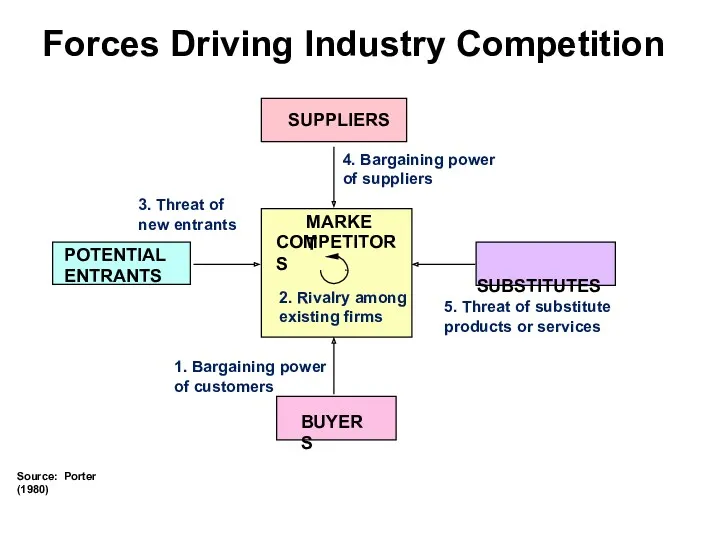
- 4. BUYERS 3. Threat of new entrants MARKET COMPETITORS 1. Bargaining power of customers SUPPLIERS SUBSTITUTES 2.
- 5. The previous lecture illustrated the impact of two of Porter’s “Five Forces of Competition”: Bargaining Power
- 6. Let’s begin with the two forces implicit in the examples from last time. According to Porter
- 7. What will be the price (P) of the “product”? How much value (V) is created? Who
- 8. What will be the price (P) of the “product”? How much value (V) is created? Who
- 9. What will be the price of the “product”? How much value is created? Who captures that
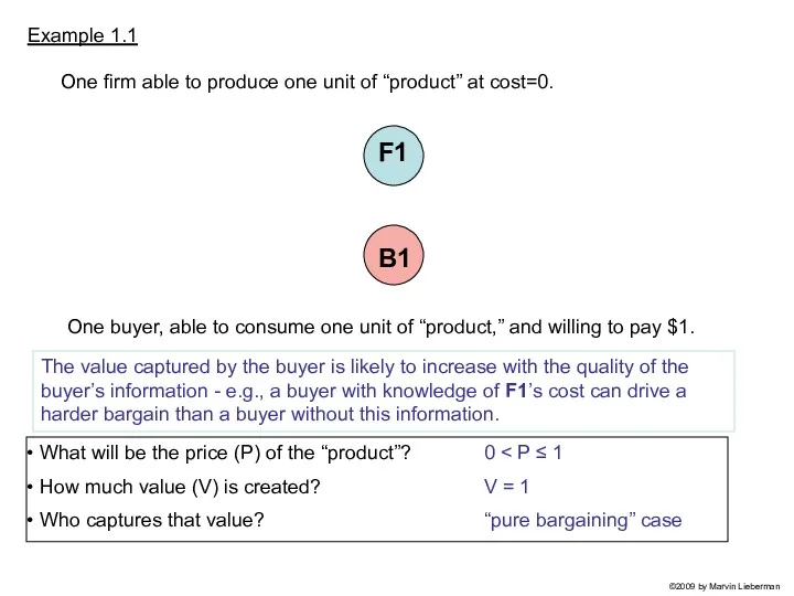
- 10. Buyer power greater when: Buyers are more concentrated Buyers are better informed Implications ©2009 by Marvin
- 11. We also saw that an increase in producer rivalry makes the industry less attractive. Consider examples
- 12. Example 1.6 What will be the price of the “product”? How much value is created? Who
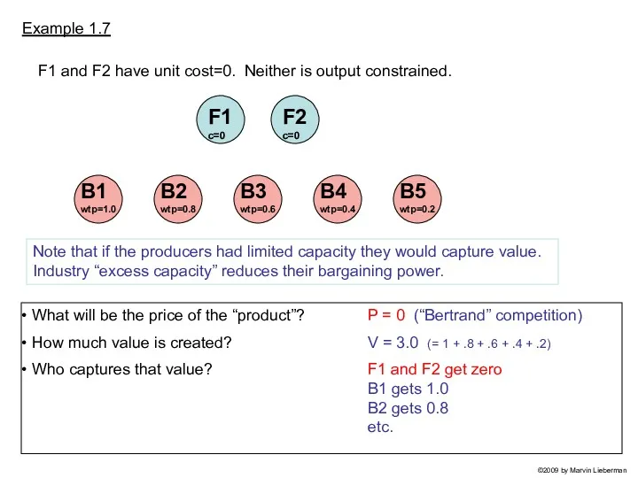
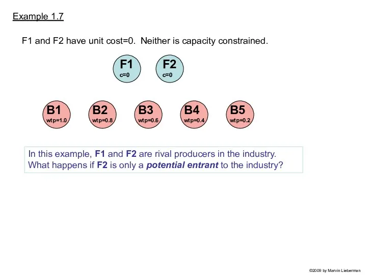
- 13. Example 1.7 What will be the price of the “product”? How much value is created? Who
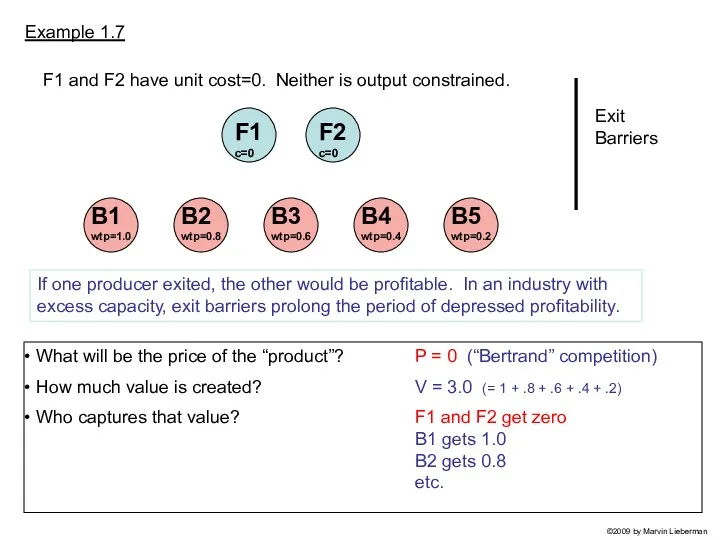
- 14. Example 1.7 What will be the price of the “product”? How much value is created? Who
- 15. Example 1.7 What will be the price of the “product”? How much value is created? Who
- 16. Implications More direct competitors Industry excess capacity Exit barriers Rivalry increases with: ©2009 by Marvin Lieberman
- 17. Now let’s consider the threat of entry. ©2009 by Marvin Lieberman
- 18. Example 1.7 F1 c=0 F2 c=0 F1 and F2 have unit cost=0. Neither is capacity constrained.
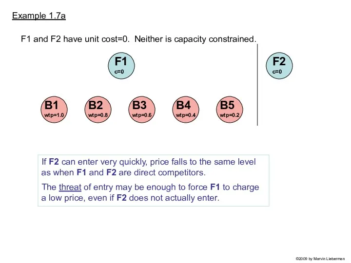
- 19. Example 1.7a F1 c=0 F1 and F2 have unit cost=0. Neither is capacity constrained. If F2
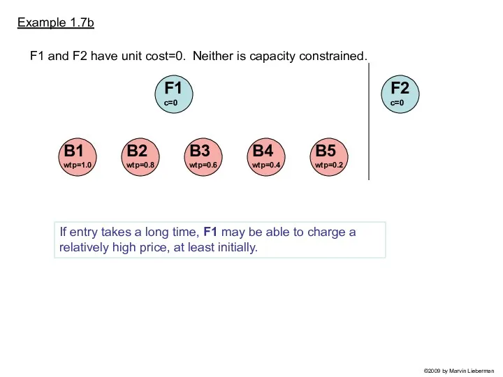
- 20. Example 1.7b F1 c=0 F1 and F2 have unit cost=0. Neither is capacity constrained. If entry
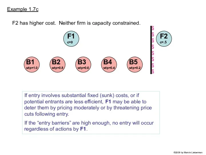
- 21. Example 1.7c F1 c=0 F2 has higher cost. Neither firm is capacity constrained. If entry involves
- 22. Potential Entrants Almost like rival producers (when entry is fast) Impeded by “entry barriers” (costs of
- 23. Now let’s consider the impact of “supplier power.” We will add supplier(s) as an additional level
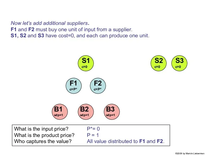
- 24. New Example. F1 and F2 have cost=0 and each can produce one unit. B1, B2 and
- 25. What is the input price (P*)? What is the product price? Who captures the value? P*=
- 26. What is the input price? What is the product price? Who captures the value? P*= 0
- 27. Implications Suppliers can siphon value from producers Power increases with supplier concentration Analysis similar to buyer
- 28. Application One example of a supplier with market power is Microsoft, whose “Windows” software has long
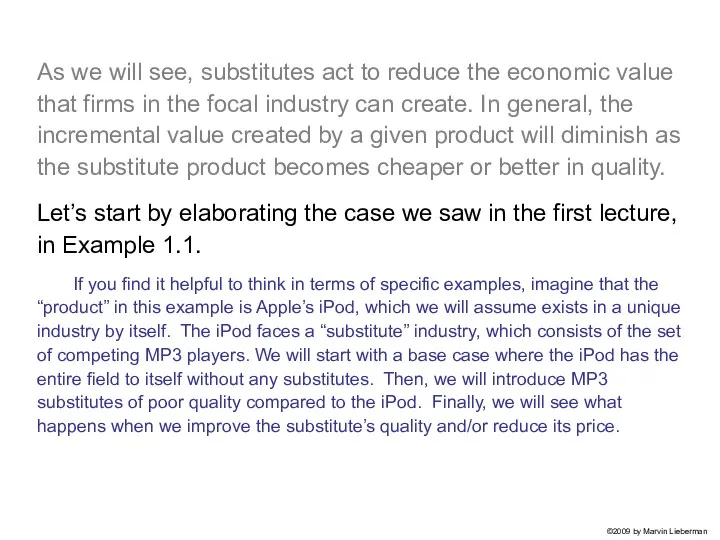
- 29. As we will see, substitutes act to reduce the economic value that firms in the focal
- 30. As we will see, substitutes act to reduce the economic value that firms in the focal
- 31. One buyer, able to consume one unit of “product,” and willing to pay $1. B1 F1
- 32. One firm able to produce one unit of “product” at cost=0. Example 1.1a. Let’s introduce a
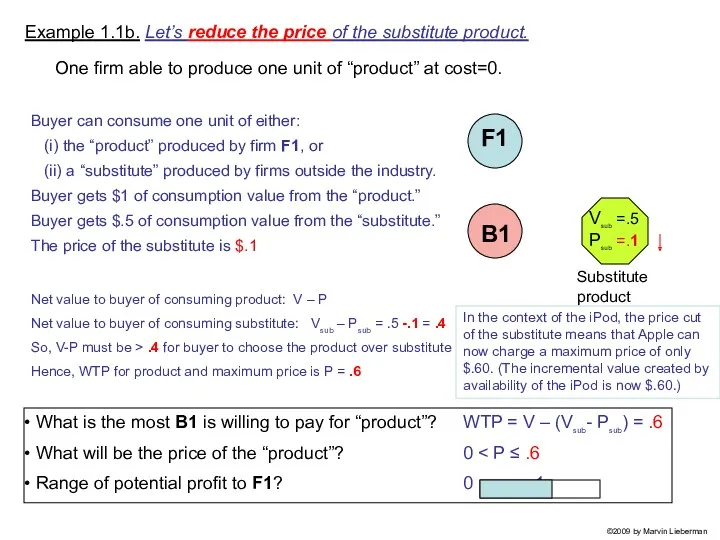
- 33. One firm able to produce one unit of “product” at cost=0. Example 1.1b. Let’s reduce the
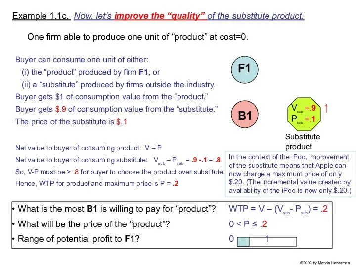
- 34. One firm able to produce one unit of “product” at cost=0. Example 1.1c. Now, let’s improve
- 35. Competition from Substitutes Reduces buyers’ WTP for the industry’s product. Strengthens bargaining position of single buyer.
- 36. Impact of Complements Sometimes called the “sixth industry force.” Can be viewed as opposite of substitutes.
- 37. Conclusions Bargaining Power of Buyers Rivalry Between Established Competitors Threat of Entry Bargaining Power of Suppliers
- 38. Conclusions The examples here have been relatively simple, but they illustrate the basic operation of the
- 40. Скачать презентацию
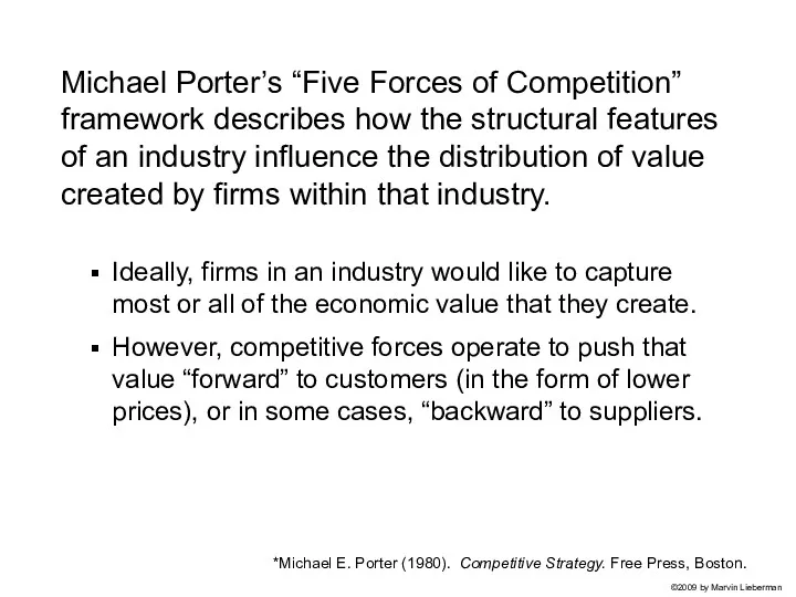
Ideally, firms in an industry would like to capture most or
Ideally, firms in an industry would like to capture most or
Michael Porter developed his Five Forces concept from basic ideas in
Michael Porter developed his Five Forces concept from basic ideas in
BUYERS
3. Threat of
new entrants
MARKET
COMPETITORS
1. Bargaining power
of customers
SUPPLIERS
BUYERS
3. Threat of
new entrants
MARKET
COMPETITORS
1. Bargaining power
of customers
SUPPLIERS
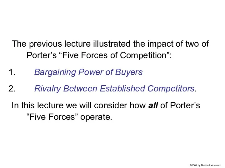
The previous lecture illustrated the impact of two of Porter’s “Five
The previous lecture illustrated the impact of two of Porter’s “Five
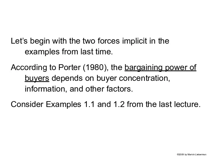
Let’s begin with the two forces implicit in the examples from
Let’s begin with the two forces implicit in the examples from
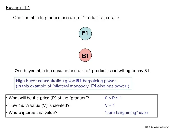
What will be the price (P) of the “product”?
How
What will be the price (P) of the “product”?
How
What will be the price (P) of the “product”?
How
What will be the price (P) of the “product”?
How
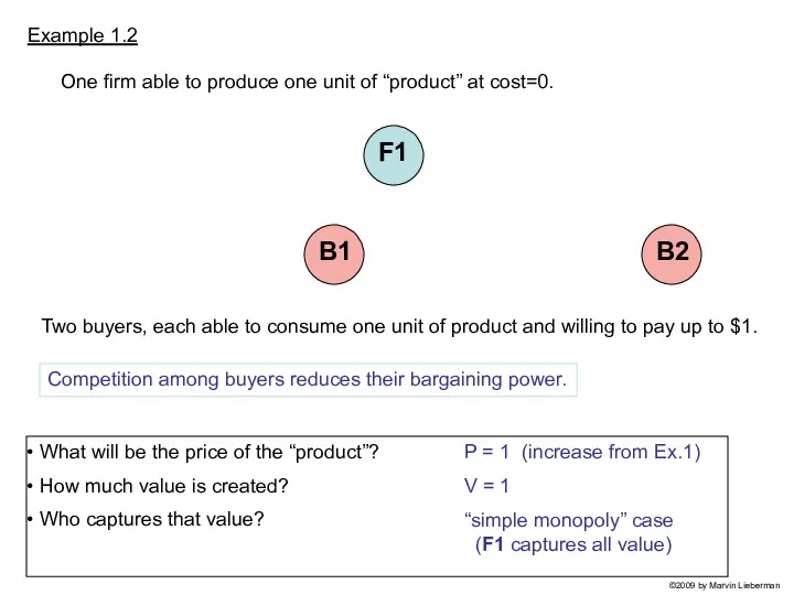
What will be the price of the “product”?
How much
What will be the price of the “product”?
How much
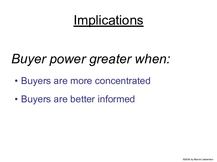
Buyer power greater when:
Buyers are more concentrated
Buyers are better informed
Implications
©2009 by
Buyer power greater when:
Buyers are more concentrated
Buyers are better informed
Implications
©2009 by
We also saw that an increase in producer rivalry makes the
We also saw that an increase in producer rivalry makes the
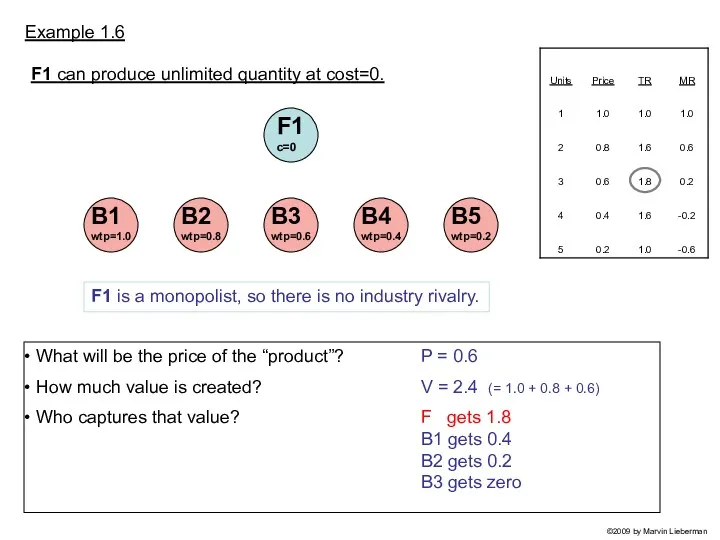
Example 1.6
What will be the price of the “product”?
Example 1.6
What will be the price of the “product”?
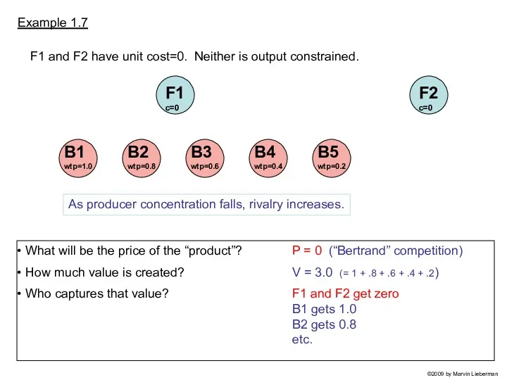
Example 1.7
What will be the price of the “product”?
Example 1.7
What will be the price of the “product”?
Example 1.7
What will be the price of the “product”?
Example 1.7
What will be the price of the “product”?
Example 1.7
What will be the price of the “product”?
Example 1.7
What will be the price of the “product”?
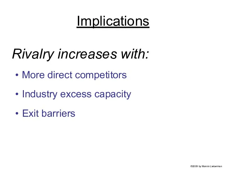
Implications
More direct competitors
Industry excess capacity
Exit barriers
Rivalry increases with:
©2009 by Marvin
Implications
More direct competitors
Industry excess capacity
Exit barriers
Rivalry increases with:
©2009 by Marvin
Now let’s consider the threat of entry.
©2009 by Marvin Lieberman
Now let’s consider the threat of entry.
©2009 by Marvin Lieberman
Example 1.7
F1 c=0
F2
c=0
F1 and F2 have unit cost=0. Neither is
Example 1.7
F1 c=0
F2
c=0
F1 and F2 have unit cost=0. Neither is
Example 1.7a
F1 c=0
F1 and F2 have unit cost=0. Neither is
Example 1.7a
F1 c=0
F1 and F2 have unit cost=0. Neither is
Example 1.7b
F1 c=0
F1 and F2 have unit cost=0. Neither is
Example 1.7b
F1 c=0
F1 and F2 have unit cost=0. Neither is
Example 1.7c
F1 c=0
F2 has higher cost. Neither firm is capacity
Example 1.7c
F1 c=0
F2 has higher cost. Neither firm is capacity
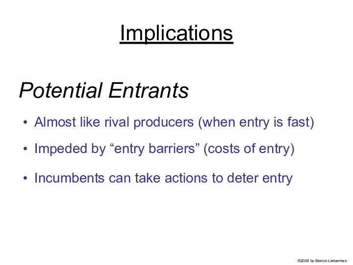
Potential Entrants
Almost like rival producers (when entry is fast)
Impeded by “entry
Potential Entrants
Almost like rival producers (when entry is fast)
Impeded by “entry
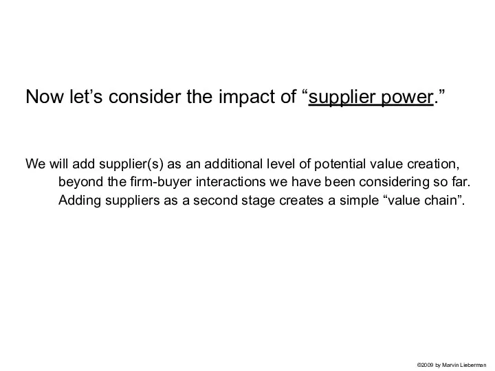
Now let’s consider the impact of “supplier power.”
We will add
Now let’s consider the impact of “supplier power.”
We will add
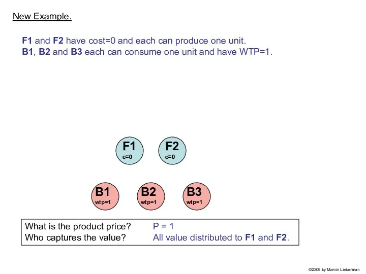
New Example.
F1 and F2 have cost=0 and each can produce
New Example.
F1 and F2 have cost=0 and each can produce
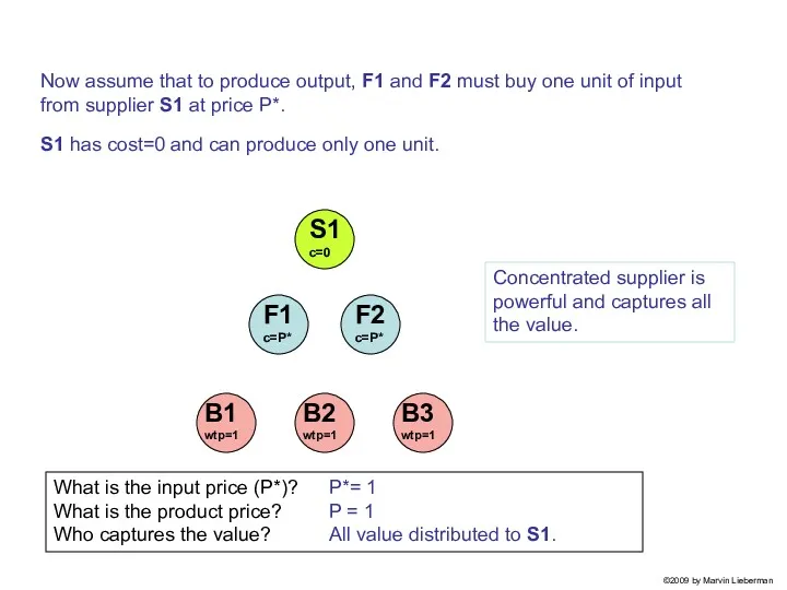
What is the input price (P*)?
What is the product price?
Who
What is the input price (P*)? What is the product price? Who
What is the input price?
What is the product price?
Who captures
What is the input price? What is the product price? Who captures
Implications
Suppliers can siphon value from producers
Power increases with supplier concentration
Analysis
Implications
Suppliers can siphon value from producers
Power increases with supplier concentration
Analysis
Application
One example of a supplier with market power is Microsoft, whose
Application
One example of a supplier with market power is Microsoft, whose
As we will see, substitutes act to reduce the economic value
As we will see, substitutes act to reduce the economic value
As we will see, substitutes act to reduce the economic value
As we will see, substitutes act to reduce the economic value
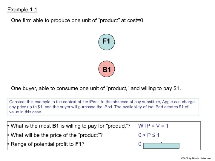
One buyer, able to consume one unit of “product,” and willing
One buyer, able to consume one unit of “product,” and willing
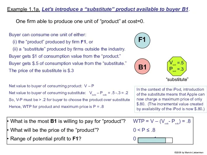
One firm able to produce one unit of “product” at cost=0.
Example
One firm able to produce one unit of “product” at cost=0.
Example
One firm able to produce one unit of “product” at cost=0.
Example
One firm able to produce one unit of “product” at cost=0.
Example
One firm able to produce one unit of “product” at cost=0.
Example
One firm able to produce one unit of “product” at cost=0.
Example
Competition from Substitutes
Reduces buyers’ WTP for the industry’s product.
Strengthens bargaining position
Competition from Substitutes
Reduces buyers’ WTP for the industry’s product.
Strengthens bargaining position
Impact of Complements
Sometimes called the “sixth industry force.”
Can be viewed as
Impact of Complements
Sometimes called the “sixth industry force.”
Can be viewed as
Conclusions
Bargaining Power of Buyers
Rivalry Between Established Competitors
Threat of Entry
Bargaining Power of
Conclusions
Bargaining Power of Buyers
Rivalry Between Established Competitors
Threat of Entry
Bargaining Power of
Conclusions
The examples here have been relatively simple, but they illustrate the
Conclusions
The examples here have been relatively simple, but they illustrate the
 Подборка презентаций к урокам экономики ( вторая часть )
 Зовнішньоекономічна діяльність та її роль у розвитку національної економіки
 Soft Computingga kirish
 Функционально-стоимостной анализ
 Elastyczność popytu i podaży
 Фирмы в экономике
 Субъект международного права : Республика Индия
 Бизнес – план создания спорт - бара
 Равновесие, эффективность и государство
 Организация производства на предприятии
 Международная интеграция
 Региональное управление (цели, задачи, функции)
 Основные фонды предприятия
 Қазақ қауымның дүниетанымы : қалыптасуы мен өзгеріске бейімделу
 Анализ использования трудовых ресурсов предприятия
 Рыночная экономика 8 класс
 Об’єкт, предмет і завдання дисципліни “Економіка праці й соціально-трудові відносини”
 Қр үкіметінің тұрақты экономикалық өсуді және жұмыспен қамтуды қамтамасыз етуге арналған дағдарысқа қарсы
 Матричные методы стратегического анализа
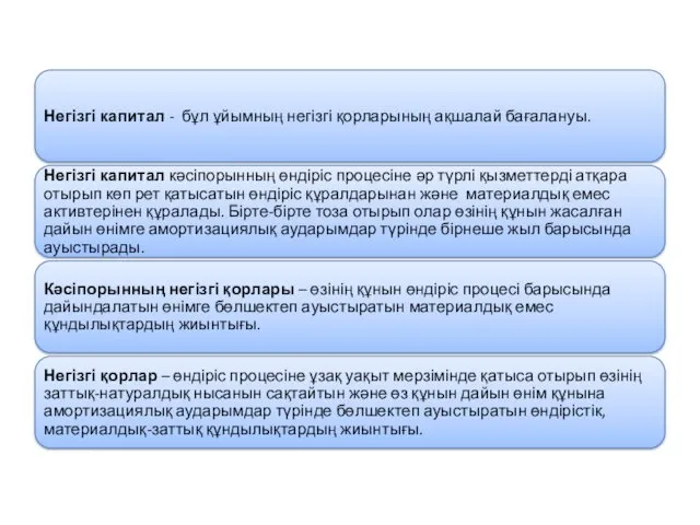 Негізгі капитал
 Инфляция и семейная экономика
 Роль экономики в жизни общества
 Показатели, которые необходимо прогнозировать в сфере потребительский рынок
 Инфляция. Определение понятия инфляция
 О мерах поддержки, предоставляемых но Фонд развития моногородов
 механизмы рынка. Тема 3-4
 Случаи несостоятельности рынка. Внешние эффекты
 Традиционный старый институционализм