- Cost-Volume-Profit (CVP) Analysis

Содержание
- 2. Basic Assumptions Changes in production/sales volume are the sole cause for cost and revenue changes Total
- 3. Basic Assumptions, continued Selling price, variable cost per unit, and fixed costs are all known and
- 4. Basic Formulae
- 5. Contribution Margin Contribution Margin equals sales less variable costs CM = S – VC Contribution Margin
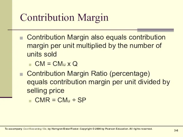
- 6. Contribution Margin Contribution Margin also equals contribution margin per unit multiplied by the number of units
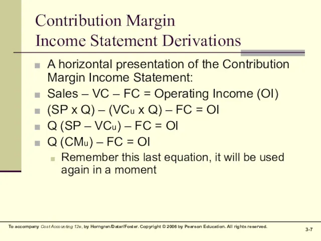
- 7. Contribution Margin Income Statement Derivations A horizontal presentation of the Contribution Margin Income Statement: Sales –
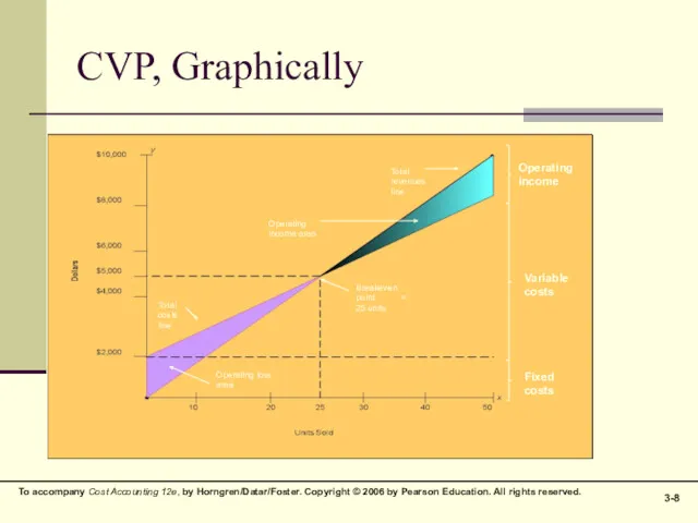
- 8. CVP, Graphically Total costs line Operating loss area Breakeven point = 25 units Total costs line
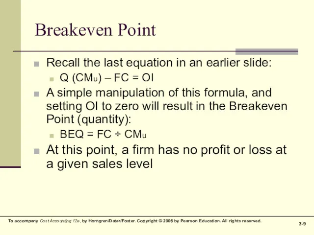
- 9. Breakeven Point Recall the last equation in an earlier slide: Q (CMu) – FC = OI
- 10. Breakeven Point, continued If per-unit values are not available, the Breakeven Point may be restated in
- 11. Breakeven Point, extended: Profit Planning With a simple adjustment, the Breakeven Point formula can be modified
- 12. CVP and Income Taxes From time to time it is necessary to move back and forth
- 13. Sensitivity Analysis CVP provides structure to answer a variety of “what-if” scenarios “What” happens to profit
- 14. Margin of Safety One indicator of risk, the Margin of Safety (MOS) measures the distance between
- 15. Operating Leverage Operating Leverage (OL) is the effect that fixed costs have on changes in operating
- 16. Effects of Sales-Mix on CVP The formulae presented to this point have assumed a single product
- 17. Effects of Sales-Mix on CVP A weighted-average CM must be calculated (in this case, for two
- 18. Multiple Cost Drivers Variable costs may arise from multiple cost drivers or activities. A separate variable
- 20. Скачать презентацию
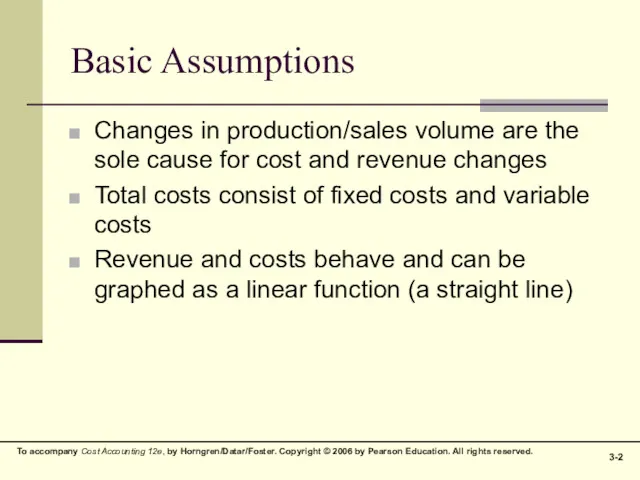
Basic Assumptions
Changes in production/sales volume are the sole cause for cost
Basic Assumptions
Changes in production/sales volume are the sole cause for cost
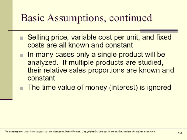
Basic Assumptions, continued
Selling price, variable cost per unit, and fixed costs
Basic Assumptions, continued
Selling price, variable cost per unit, and fixed costs
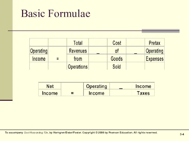
Basic Formulae
Basic Formulae
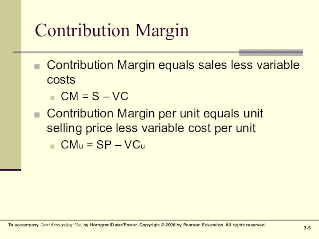
Contribution Margin
Contribution Margin equals sales less variable costs
CM = S
Contribution Margin
Contribution Margin equals sales less variable costs
CM = S
Contribution Margin
Contribution Margin also equals contribution margin per unit multiplied by
Contribution Margin
Contribution Margin also equals contribution margin per unit multiplied by
Contribution Margin
Income Statement Derivations
A horizontal presentation of the Contribution Margin
Contribution Margin
Income Statement Derivations
A horizontal presentation of the Contribution Margin
CVP, Graphically
Total costs line
Operating loss area
Breakeven point = 25 units
Total costs
CVP, Graphically
Total costs line
Operating loss area
Breakeven point = 25 units
Total costs
Breakeven Point
Recall the last equation in an earlier slide:
Q (CMu) –
Breakeven Point
Recall the last equation in an earlier slide:
Q (CMu) –
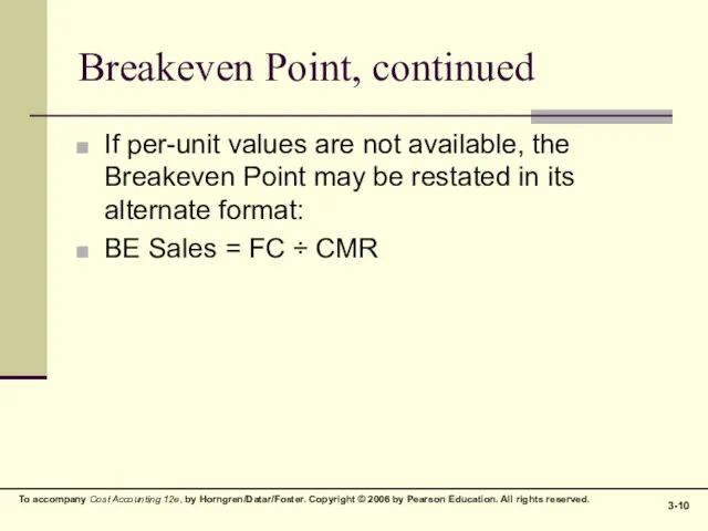
Breakeven Point, continued
If per-unit values are not available, the Breakeven Point
Breakeven Point, continued
If per-unit values are not available, the Breakeven Point
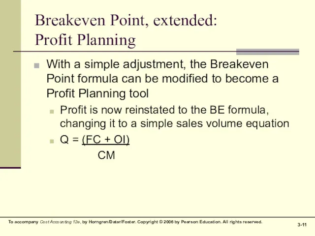
Breakeven Point, extended:
Profit Planning
With a simple adjustment, the Breakeven Point
Breakeven Point, extended:
Profit Planning
With a simple adjustment, the Breakeven Point
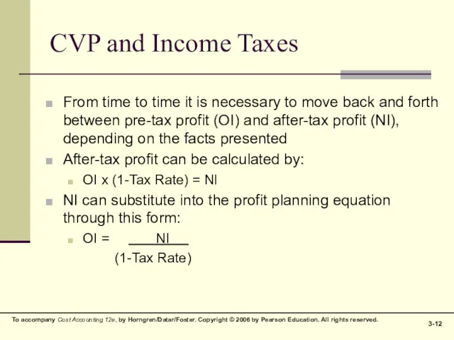
CVP and Income Taxes
From time to time it is necessary to
CVP and Income Taxes
From time to time it is necessary to
Sensitivity Analysis
CVP provides structure to answer a variety of “what-if” scenarios
“What”
Sensitivity Analysis
CVP provides structure to answer a variety of “what-if” scenarios
“What”
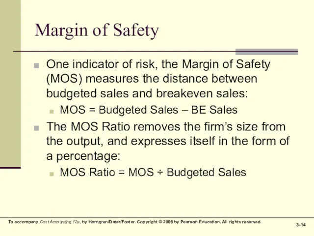
Margin of Safety
One indicator of risk, the Margin of Safety (MOS)
Margin of Safety
One indicator of risk, the Margin of Safety (MOS)
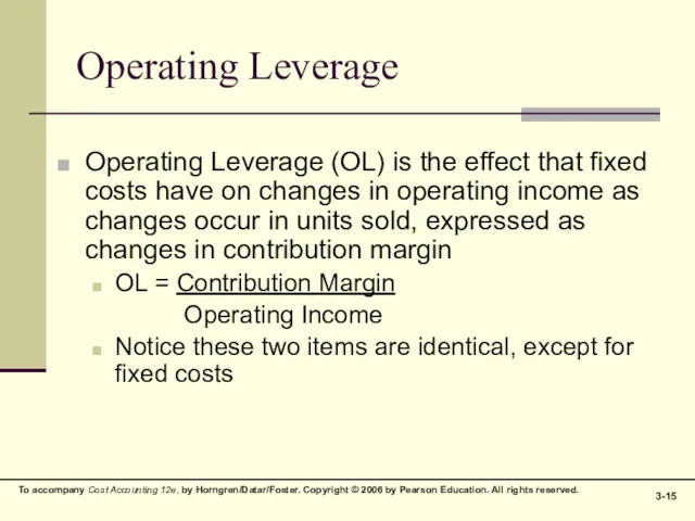
Operating Leverage
Operating Leverage (OL) is the effect that fixed costs have
Operating Leverage
Operating Leverage (OL) is the effect that fixed costs have
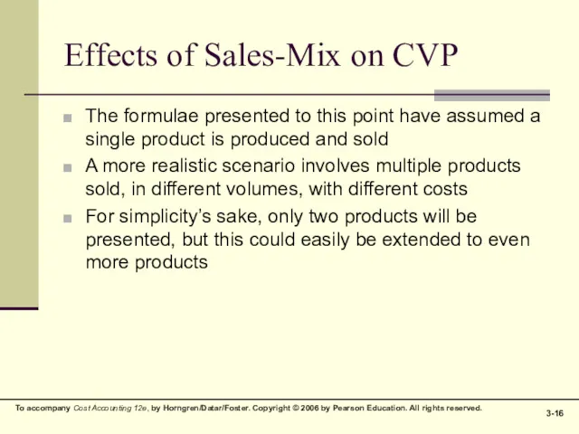
Effects of Sales-Mix on CVP
The formulae presented to this point have
Effects of Sales-Mix on CVP
The formulae presented to this point have
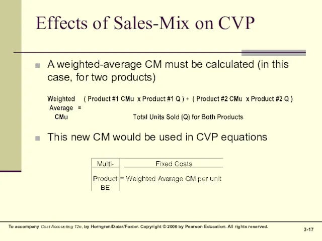
Effects of Sales-Mix on CVP
A weighted-average CM must be calculated (in
Effects of Sales-Mix on CVP
A weighted-average CM must be calculated (in
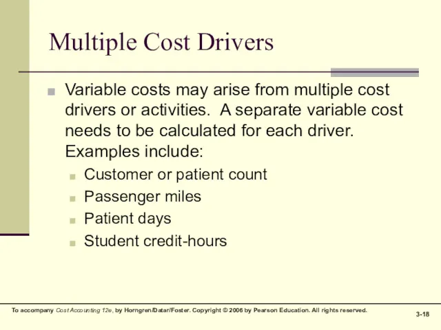
Multiple Cost Drivers
Variable costs may arise from multiple cost drivers or
Multiple Cost Drivers
Variable costs may arise from multiple cost drivers or
 Сводка и группровка статистических данных
 Салықтар және салық салу. Тақырып 6
 Сборы за пользование объектами животного мира и за пользование объектами водных биологических ресурсов
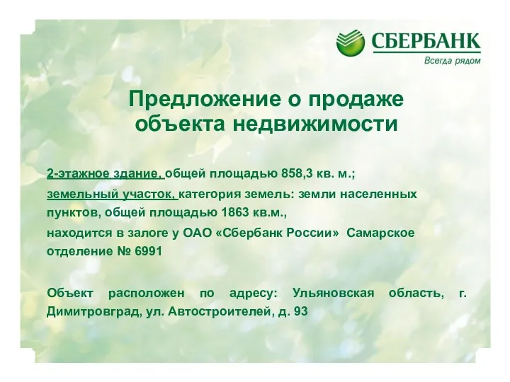 Предложение о продаже объекта недвижимости
 Электронные деньги
 Міжнародний рух інвестиційного капіталу та виробнича діяльність
 Понятие и виды прибыли
 Бухгалтерське законодавство та особливості обліку у Франції
 Витрати виробництва та витрати операційної діяльності (тема 4)
 Себестоимость. Учет затрат на производство и реализацию продукции и калькулирование себестоимости продукции
 Исполнение обязанности по уплате налогов и сборов
 Диагностика финансово-хозяйственной деятельности ПАО Челябинский металлургический комбинат
 Анализ финансовых результатов деятельности предприятия ФГУП ФЯО ГХК
 Учет и аудит собственного капитала и резервов
 Пусть ваши деньги работают Version 2.6 Euro
 Понятие ценных бумаг
 Косвенные налоги. Налог на добавленную стоимость (НДС) (глава 21 НК РФ)
 Финансовые рынки и институты
 T2_L10
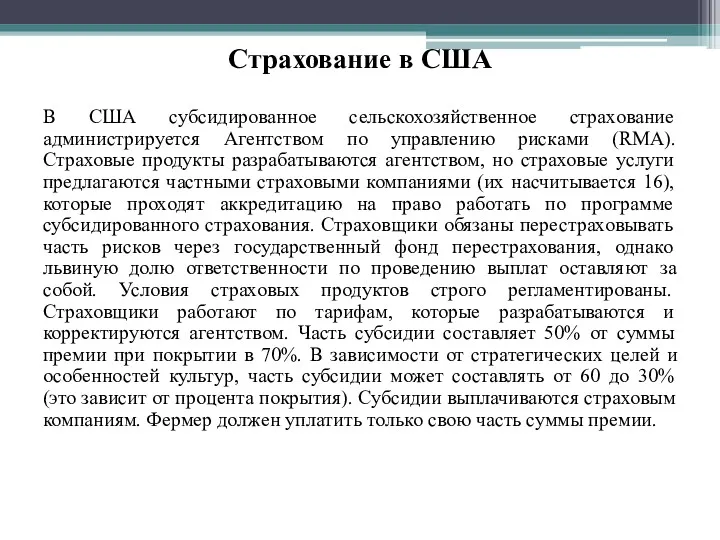 Субсидированное сельскохозяйственное страхование в США
 Распределение, неравенство доходов. Перераспределение
 Анализ ликвидности бухгалтерского баланса
 Финансовая система
 Небольшой опрос по прошедшим темам
 Деньги: причины возникновения, формы и функции
 Налог на доходы физических лиц
 Виды кредитов
 Валютное регулирование и валютный контроль. Лекция 2 - Валютное регулирование