- Dynamic models and the Kalman filter

Содержание
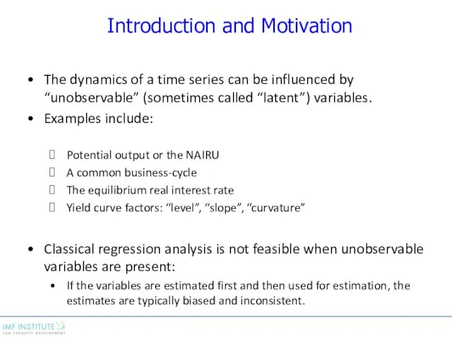
- 2. Introduction and Motivation The dynamics of a time series can be influenced by “unobservable” (sometimes called
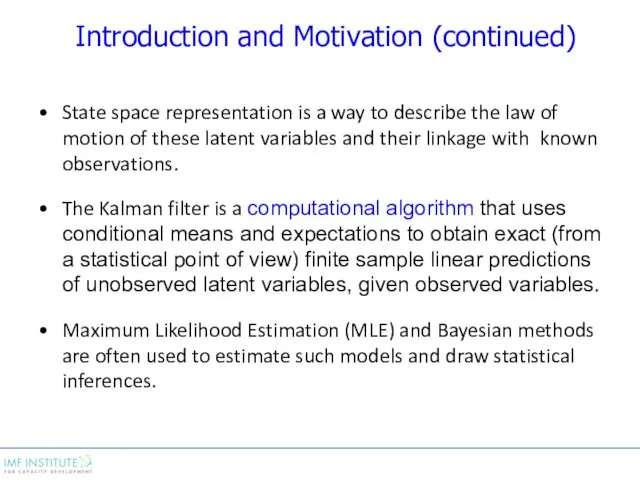
- 3. Introduction and Motivation (continued) State space representation is a way to describe the law of motion
- 4. Common Usage of These Techniques Macroeconomics, finance, time series models Autopilot, radar tracking Orbit tracking, satellite
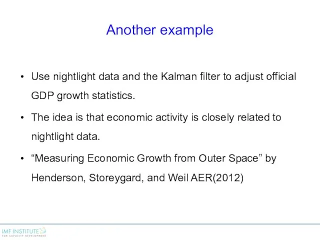
- 5. Another example Use nightlight data and the Kalman filter to adjust official GDP growth statistics. The
- 6. Measuring Long-Term Growth
- 7. Measuring Short-Term Growth
- 8. Measuring Short-Term Growth
- 9. Content Outline: Lecture Segments State Space Representation The Kalman Filter Maximum Likelihood Estimation and Kalman Smoothing
- 10. Content Outline: Workshops Workshops Estimation of equilibrium real interest rate, trend growth rate, and potential output
- 11. State Space Representation
- 12. Basic Setup Let yt be an (or a vector) observable variable(s) at time t. E.g., return
- 13. Basic Setup The state-space representation of the dynamics of yt is given by : We assume
- 14. Basic Setup The state-space representation of the dynamics of yt is given by : with The
- 15. Basic Setup The error terms in the two equations are such that: State equation Observation equation
- 16. What if you know that are serially correlated: and , Then so one of the assumptions
- 17. The State Space Representation: Examples Example #1: simple version of the CAPM st one variable, return
- 18. Example #2: growth and real business cycle (small open economy with a large export sector) st
- 19. Example #3: interest rates on zero-coupon bonds of different maturity st one variable, latent variable yt
- 20. Example #4: an AR(2) process Can we still apply the state space representation? Yes! Consider the
- 21. Example #4: an AR(2) process The state equation: And the observation equation: What are matrices Ω
- 22. Consider the same AR(2) process Another possible state equation: And the corresponding observation equation: These two
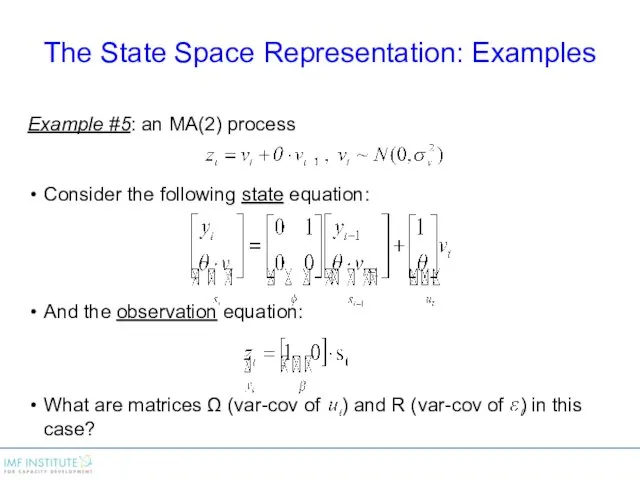
- 23. Example #5: an MA(2) process Consider the following state equation: And the observation equation: What are
- 24. Example #5: an MA(2) process Consider the following state equation: And the observation equation: What are
- 25. Example #6: A random walk plus drift process State equation? Observation equation? What are the loadings
- 26. In this course we will deal only with stable systems: Such systems that for any initial
- 27. The Kalman Filter
- 28. State Space Representation [univariate case]: Notation: is the best linear predictor of st conditional on the
- 29. Kalman Filter: Main Idea Moving from t-1 to t Suppose we know and at time t-1.
- 30. Kalman Filter: Main Idea How to update st|t ? Idea: use the observed prediction error to
- 31. Kalman Filter: More Notations is the prediction error variance of given the history of observed variables
- 32. Kalman Gain: Intuition Kalman gain is chosen so that is minimized. It can be shown that
- 33. Kalman Filter: Example Kalman gain is Consider State equation Observation equation Additionally , where is a
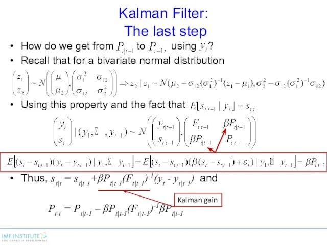
- 34. Kalman Filter: The last step How do we get from to using ? Recall that for
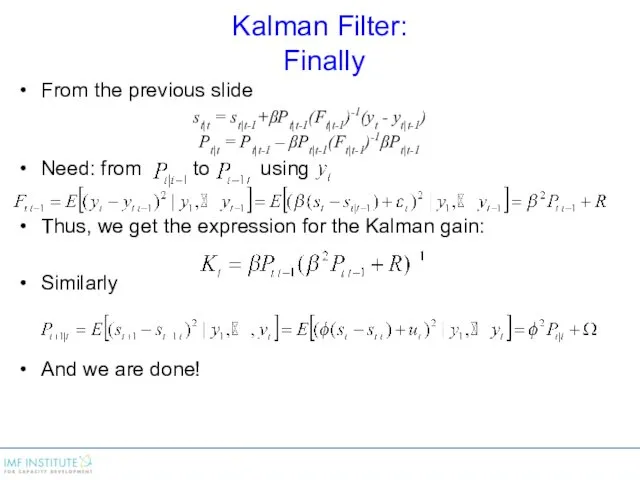
- 35. Kalman Filter: Finally From the previous slide st|t = st|t-1+βPt|t-1(Ft|t-1)-1(yt - yt|t-1) Pt|t = Pt|t-1 –
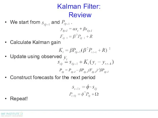
- 36. Kalman Filter: Review We start from and . yt|t-1 = αxt + βst|t-1 Calculate Kalman gain
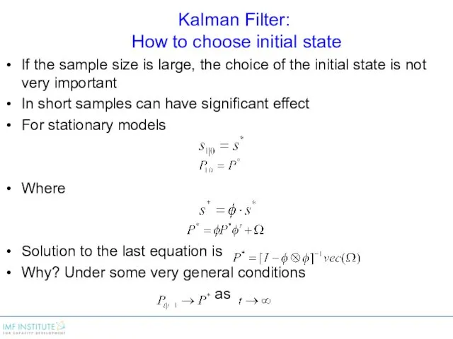
- 37. Kalman Filter: How to choose initial state If the sample size is large, the choice of
- 38. Kalman Filter as a Recursive Regression Consider a regular regression function where Substituting From one of
- 39. Kalman Filter as a Recursive Regression Consider a regular regression function where Substituting From one of
- 40. Kalman Filter as a Recursive Regression Thus the Kalman filter can be interpreted as a recursive
- 41. Optimality of the Kalman Filter Using the property of OLS estimates that constructed residuals are uncorrelated
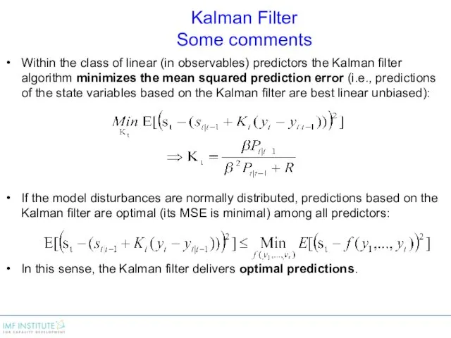
- 42. Kalman Filter Some comments Within the class of linear (in observables) predictors the Kalman filter algorithm
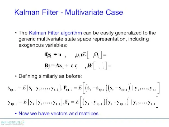
- 43. Kalman Filter - Multivariate Case The Kalman Filter algorithm can be easily generalized to the generic
- 44. Kalman Filter Algorithm – Multivariate Case
- 45. Kalman Filter Algorithm – Multivariate Case (cont.)
- 46. Kalman Filter Algorithm – Multivariate Case (cont.)
- 47. ML Estimation and Kalman Smoothing
- 48. Maximum Likelihood Estimation The algorithm in the previous section assumes knowledge of the parameters. If these
- 49. To estimate model parameters through maximizing log-likelihood: Step 1: For every set of the underlying parameters,
- 50. Kalman Smoothing For each period t, the Kalman filter uses only information available up to time
- 51. Kalman Smoothing Using the same principles for normal conditional distribution, it is possible to show that
- 53. Скачать презентацию
Introduction and Motivation
The dynamics of a time series can be influenced
Introduction and Motivation
The dynamics of a time series can be influenced
Introduction and Motivation (continued)
State space representation is a way to describe
Introduction and Motivation (continued)
State space representation is a way to describe
Common Usage of These Techniques
Macroeconomics, finance, time series models
Autopilot, radar tracking
Orbit
Common Usage of These Techniques
Macroeconomics, finance, time series models
Autopilot, radar tracking
Orbit
Another example
Use nightlight data and the Kalman filter to adjust official
Another example
Use nightlight data and the Kalman filter to adjust official
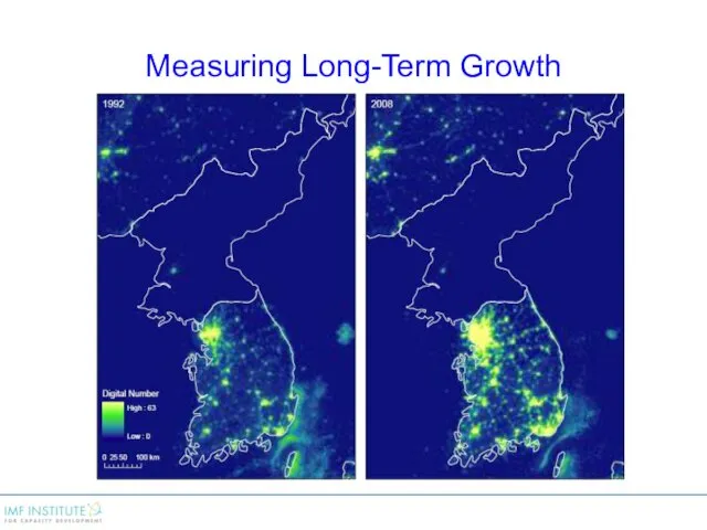
Measuring Long-Term Growth
Measuring Long-Term Growth
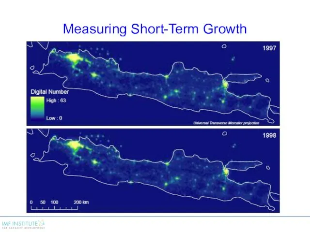
Measuring Short-Term Growth
Measuring Short-Term Growth
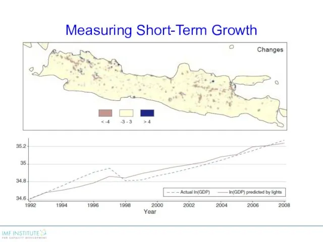
Measuring Short-Term Growth
Measuring Short-Term Growth
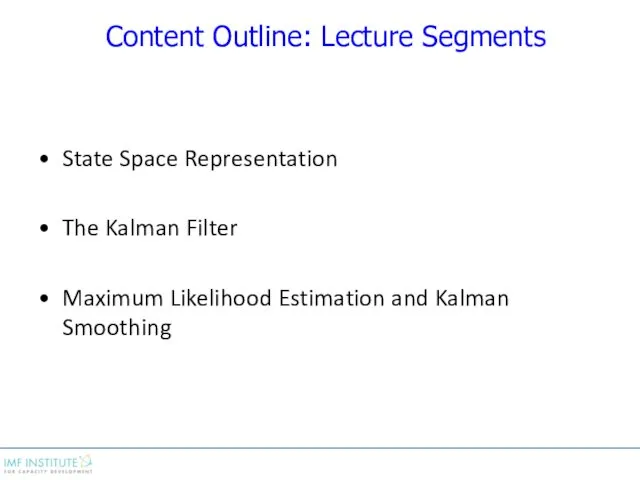
Content Outline: Lecture Segments
State Space Representation
The Kalman Filter
Maximum Likelihood Estimation and
Content Outline: Lecture Segments
State Space Representation
The Kalman Filter
Maximum Likelihood Estimation and
Content Outline: Workshops
Workshops
Estimation of equilibrium real interest rate, trend growth rate,
Content Outline: Workshops
Workshops
Estimation of equilibrium real interest rate, trend growth rate,

State Space Representation
State Space Representation
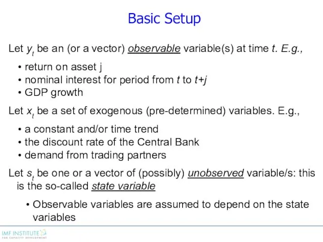
Basic Setup
Let yt be an (or a vector) observable variable(s) at
Basic Setup
Let yt be an (or a vector) observable variable(s) at
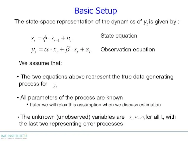
Basic Setup
The state-space representation of the dynamics of yt is given
Basic Setup
The state-space representation of the dynamics of yt is given
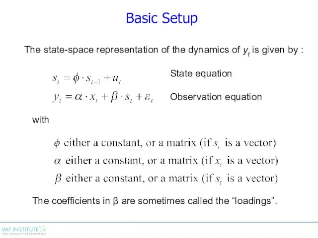
Basic Setup
The state-space representation of the dynamics of yt is given
Basic Setup
The state-space representation of the dynamics of yt is given
Basic Setup
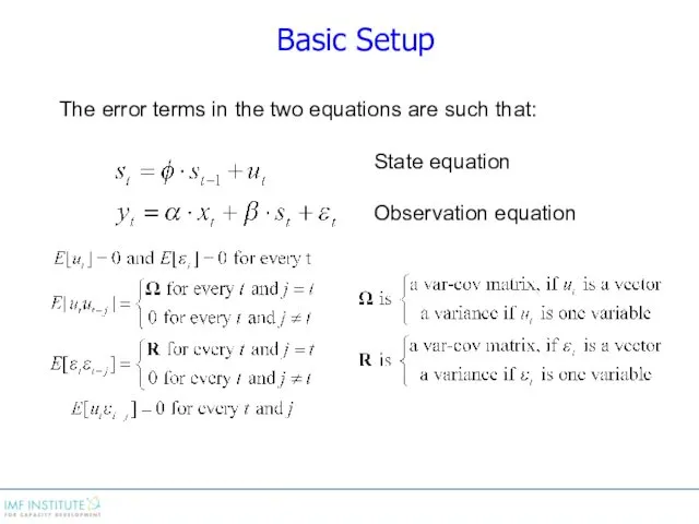
The error terms in the two equations are such that:
State
Basic Setup
The error terms in the two equations are such that:
State
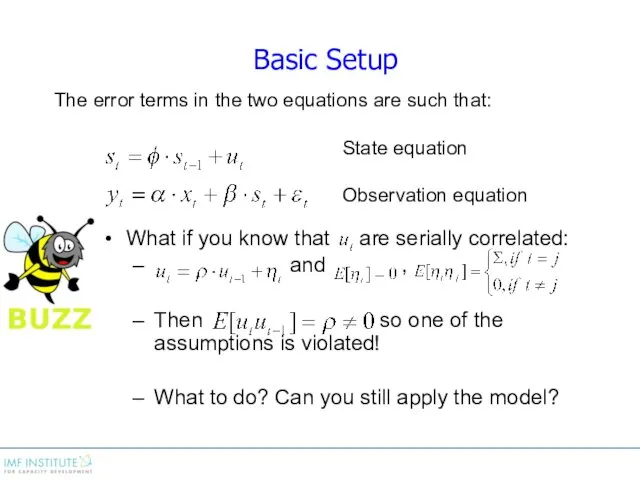
What if you know that are serially correlated:
and ,
What if you know that are serially correlated:
and ,
The State Space Representation: Examples
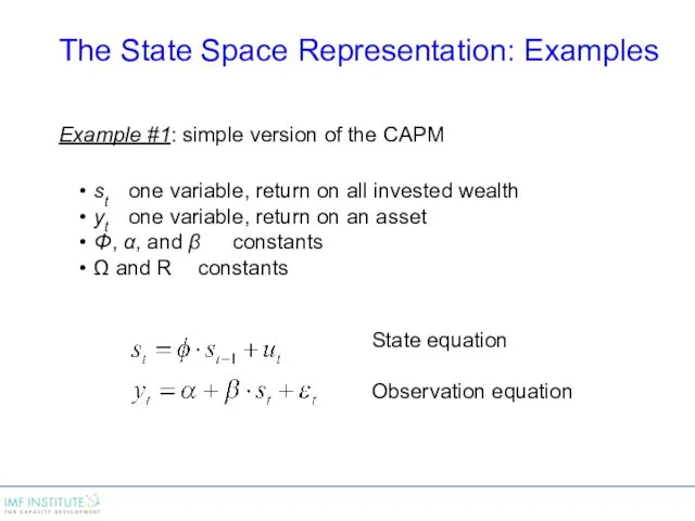
Example #1: simple version of the CAPM
st one
The State Space Representation: Examples
Example #1: simple version of the CAPM
st one
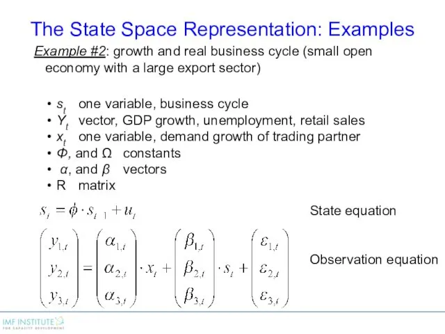
Example #2: growth and real business cycle (small open economy with
Example #2: growth and real business cycle (small open economy with
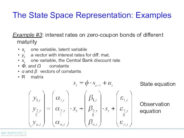
Example #3: interest rates on zero-coupon bonds of different maturity
st one variable,
Example #3: interest rates on zero-coupon bonds of different maturity
st one variable,
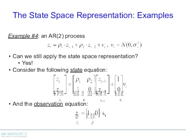
Example #4: an AR(2) process
Can we still apply the state space
Example #4: an AR(2) process
Can we still apply the state space
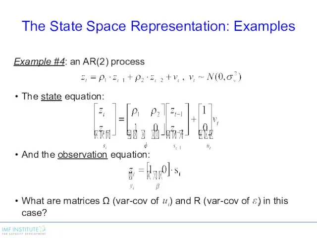
Example #4: an AR(2) process
The state equation:
And the observation equation:
What are
Example #4: an AR(2) process
The state equation:
And the observation equation:
What are
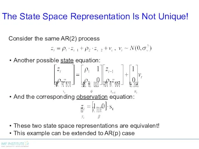
Consider the same AR(2) process
Another possible state equation:
And the corresponding observation
Consider the same AR(2) process
Another possible state equation:
And the corresponding observation
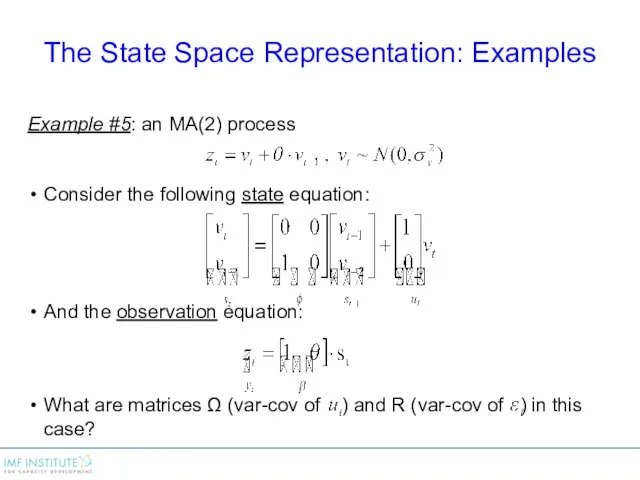
Example #5: an MA(2) process
Consider the following state equation:
And the observation
Example #5: an MA(2) process
Consider the following state equation:
And the observation
Example #5: an MA(2) process
Consider the following state equation:
And the observation
Example #5: an MA(2) process
Consider the following state equation:
And the observation
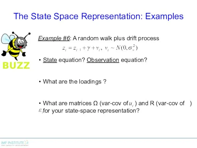
Example #6: A random walk plus drift process
State equation? Observation equation?
What
Example #6: A random walk plus drift process
State equation? Observation equation?
What
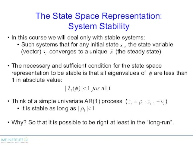
In this course we will deal only with stable systems:
Such systems
In this course we will deal only with stable systems:
Such systems

The Kalman Filter
The Kalman Filter
![State Space Representation [univariate case]: Notation: is the best linear](/_ipx/f_webp&q_80&fit_contain&s_1440x1080/imagesDir/jpg/96593/slide-27.jpg)
State Space Representation [univariate case]:
Notation:
is the best linear predictor
State Space Representation [univariate case]:
Notation:
is the best linear predictor
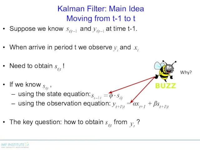
Kalman Filter: Main Idea
Moving from t-1 to t
Suppose we know
Kalman Filter: Main Idea
Moving from t-1 to t
Suppose we know
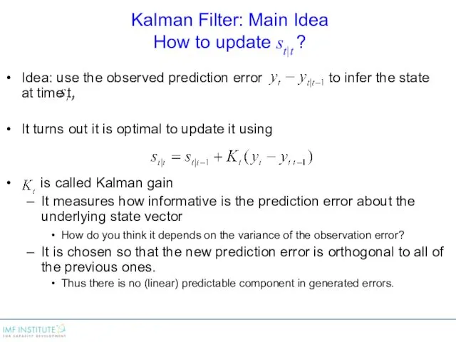
Kalman Filter: Main Idea
How to update st|t ?
Idea: use the observed
Kalman Filter: Main Idea
How to update st|t ?
Idea: use the observed
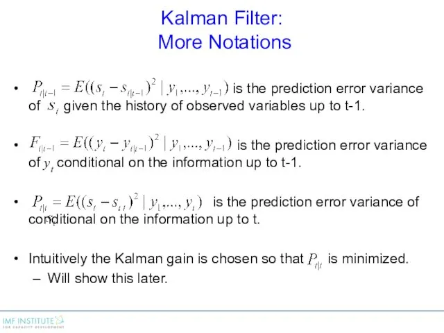
Kalman Filter:
More Notations
is the prediction error variance of given
Kalman Filter:
More Notations
is the prediction error variance of given

Kalman Gain:
Intuition
Kalman gain is chosen so that is minimized.
It can be
Kalman Gain:
Intuition
Kalman gain is chosen so that is minimized.
It can be
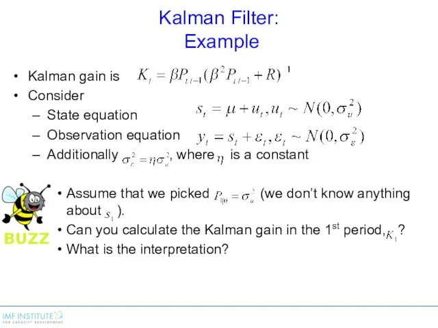
Kalman Filter:
Example
Kalman gain is
Consider
State equation
Observation equation
Additionally
Kalman Filter:
Example
Kalman gain is
Consider
State equation
Observation equation
Additionally
Kalman Filter:
The last step
How do we get from to using
Kalman Filter:
The last step
How do we get from to using
Kalman Filter:
Finally
From the previous slide
st|t = st|t-1+βPt|t-1(Ft|t-1)-1(yt - yt|t-1)
Pt|t
Kalman Filter:
Finally
From the previous slide
st|t = st|t-1+βPt|t-1(Ft|t-1)-1(yt - yt|t-1)
Pt|t
Kalman Filter:
Review
We start from and .
yt|t-1 = αxt +
Kalman Filter:
Review
We start from and .
yt|t-1 = αxt +
Kalman Filter:
How to choose initial state
If the sample size is
Kalman Filter:
How to choose initial state
If the sample size is
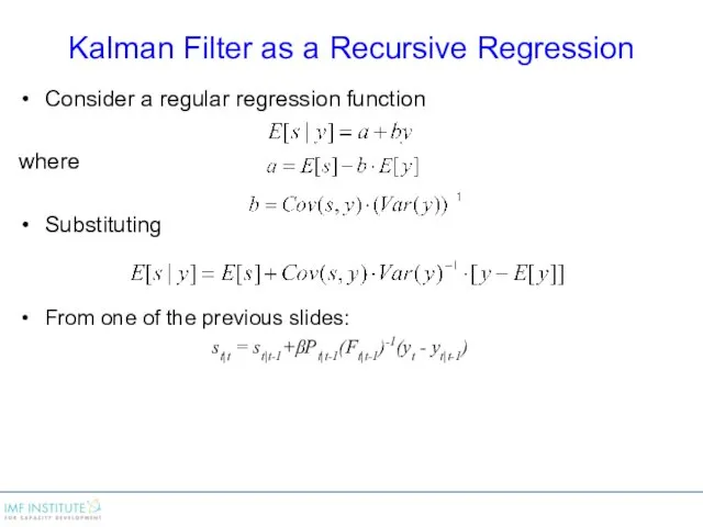
Kalman Filter as a Recursive Regression
Consider a regular regression function
where
Substituting
From
Kalman Filter as a Recursive Regression
Consider a regular regression function
where
Substituting
From
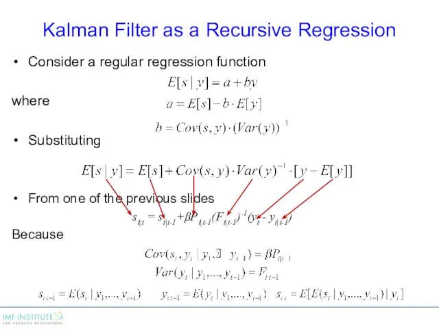
Kalman Filter as a Recursive Regression
Consider a regular regression function
where
Substituting
From
Kalman Filter as a Recursive Regression
Consider a regular regression function
where
Substituting
From
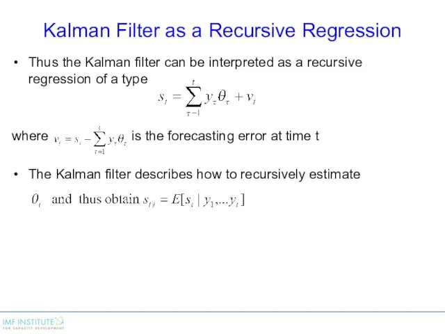
Kalman Filter as a Recursive Regression
Thus the Kalman filter can be
Kalman Filter as a Recursive Regression
Thus the Kalman filter can be
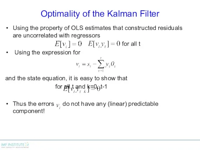
Optimality of the Kalman Filter
Using the property of OLS estimates that
Optimality of the Kalman Filter
Using the property of OLS estimates that
Kalman Filter
Some comments
Within the class of linear (in observables) predictors the
Kalman Filter
Some comments
Within the class of linear (in observables) predictors the
Kalman Filter - Multivariate Case
The Kalman Filter algorithm can be easily
Kalman Filter - Multivariate Case
The Kalman Filter algorithm can be easily
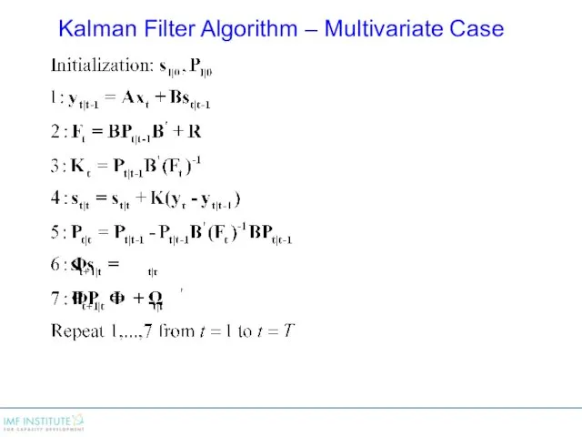
Kalman Filter Algorithm – Multivariate Case
Kalman Filter Algorithm – Multivariate Case
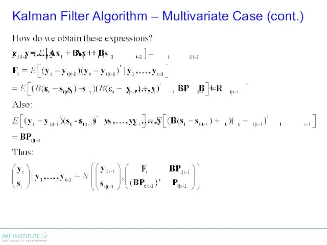
Kalman Filter Algorithm – Multivariate Case (cont.)
Kalman Filter Algorithm – Multivariate Case (cont.)

Kalman Filter Algorithm – Multivariate Case (cont.)
Kalman Filter Algorithm – Multivariate Case (cont.)
ML Estimation and Kalman Smoothing
ML Estimation and Kalman Smoothing
Maximum Likelihood Estimation
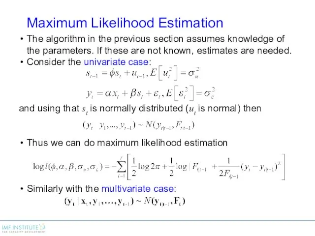
The algorithm in the previous section assumes knowledge of
Maximum Likelihood Estimation
The algorithm in the previous section assumes knowledge of
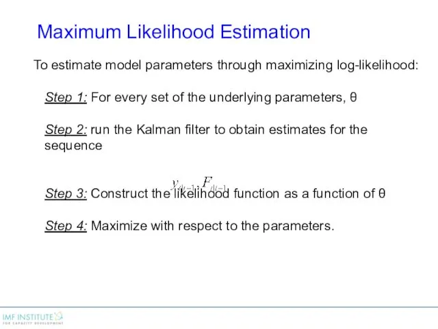
To estimate model parameters through maximizing log-likelihood:
Step 1: For every set
To estimate model parameters through maximizing log-likelihood:
Step 1: For every set
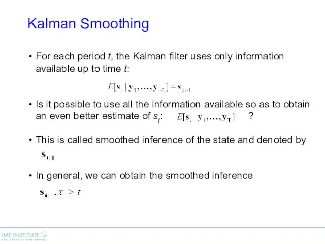
Kalman Smoothing
For each period t, the Kalman filter uses only information
Kalman Smoothing
For each period t, the Kalman filter uses only information
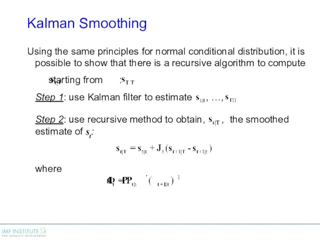
Kalman Smoothing
Using the same principles for normal conditional distribution, it is
Kalman Smoothing
Using the same principles for normal conditional distribution, it is
 Равнодействующая сил
 Protein structure: prediction engineering design
 Механика жидкостей и газов. (Лекция 9)
 Масса тела
 Ремонт автомобилей. Ремонт коленчатых валов и шатунов. (Тема 4.5)
 Техническое обслуживание рулевого управления автомобиля Toyota Mark II
 Простые механизмы в технике и в быту
 Машиноведение. История создания швейной машины
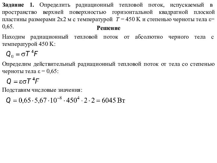 Тепловое излучение. Задачи
 Что изучает физика? Некоторые физические термины
 Прості механізми побутових пристроїв
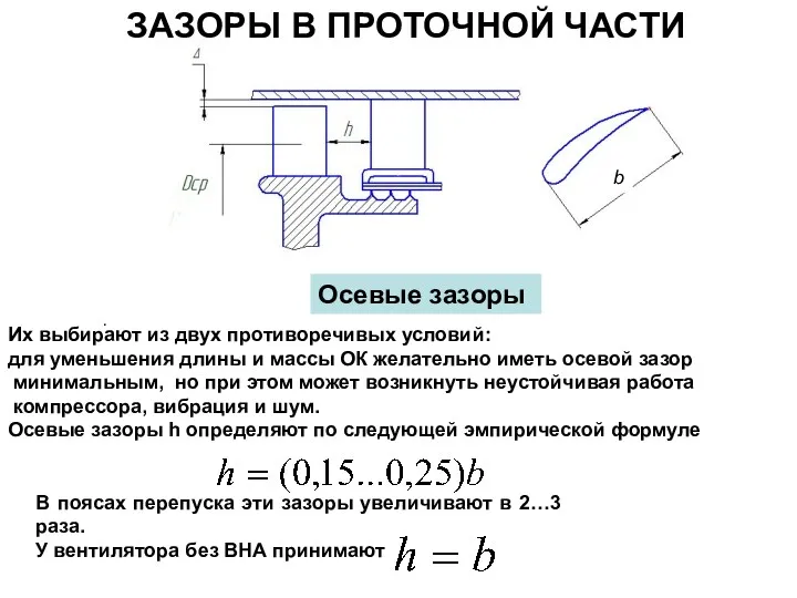 Зазоры в проточной части
 Магнитное поле. Взаимодействие токов
 Механізація подрібнення стеблових кормів
 Сила трения. Трение в природе и технике
 Ремонт авиационного оборудования с боевыми и эксплуатационными повреждениями
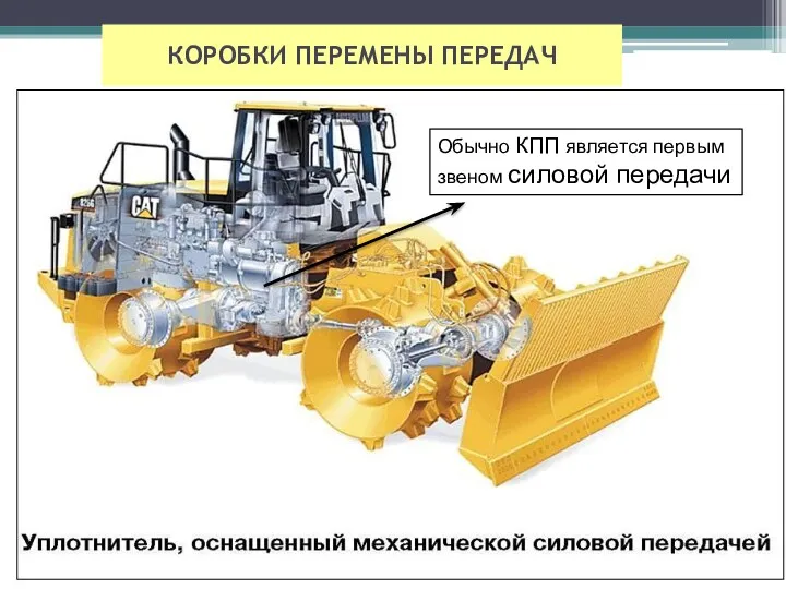 Коробки перемены передач
 Электромагнитное поле
 Физика в нашей жизни
 Влияние на работу дороги природных факторов
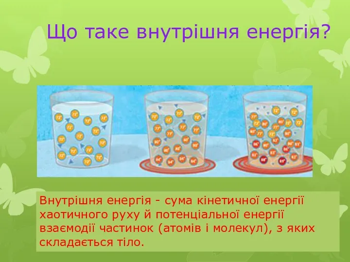 Внутрішня енергія
 Основы поверхностной обработки полупроводниковых материалов
 Урок презентация Реактивное движение
 Закон Ома на участке цепи. Диаграмма связи величин: U, I, R
 Разработка установки для замены масла в двигателе
 Закон всемирного тяготения
 Магнитное поле
 Ионизирующие излучения