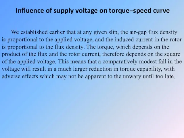
- Influence of supply voltage on torque–speed curve

Содержание
- 3. Table of synchronous speed of rotation of induction motors as a function of frequency and number
- 4. Influence of supply voltage on torque–speed curve We established earlier that at any given slip, the
- 5. To illustrate the problem, consider the torque–speed curves for a cage motor shown in Figure. The
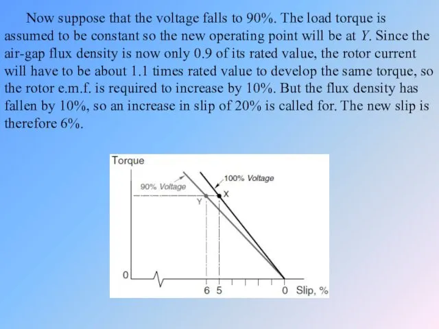
- 6. Now suppose that the voltage falls to 90%. The load torque is assumed to be constant
- 7. The drop in speed from 95% of synchronous to 94% may well not be noticed, and
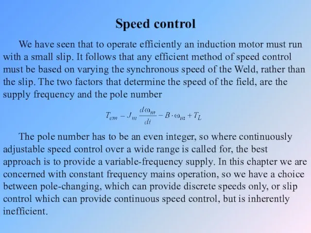
- 8. Speed control We have seen that to operate efficiently an induction motor must run with a
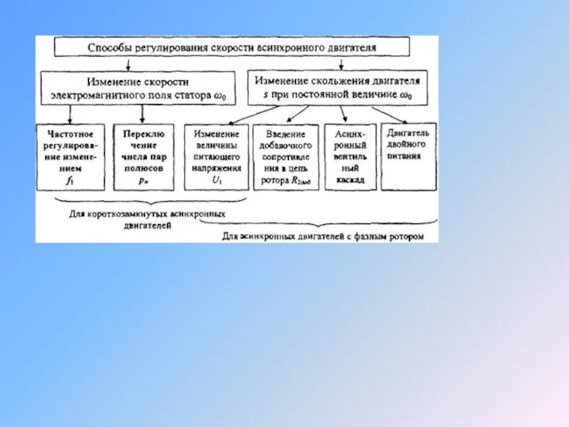
- 9. Pole-changing motors For some applications continuous speed control may be an unnecessary luxury, and it may
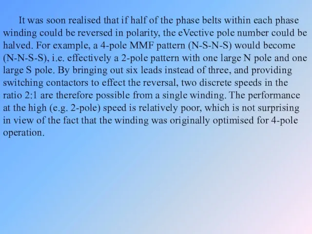
- 10. It was soon realised that if half of the phase belts within each phase winding could
- 11. It was not until the advent of the more sophisticated pole amplitude modulation (PAM) method in
- 12. The beauty of the PAM method is that it is not expensive. The stator winding has
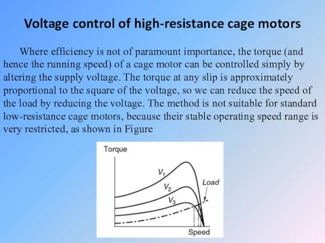
- 13. Voltage control of high-resistance cage motors Where efficiency is not of paramount importance, the torque (and
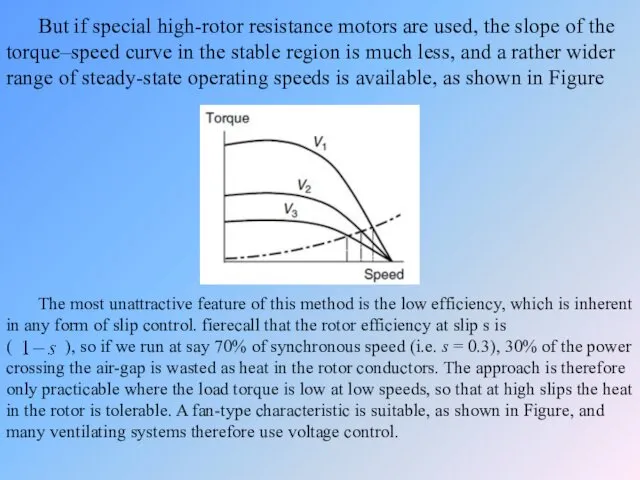
- 14. But if special high-rotor resistance motors are used, the slope of the torque–speed curve in the
- 15. Voltage control became feasible only when relatively cheap thyristor a.c. voltage regulators arrived on the scene
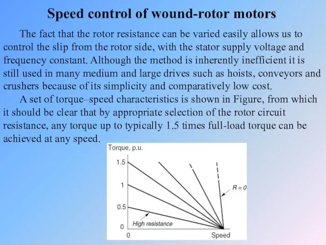
- 16. Speed control of wound-rotor motors The fact that the rotor resistance can be varied easily allows
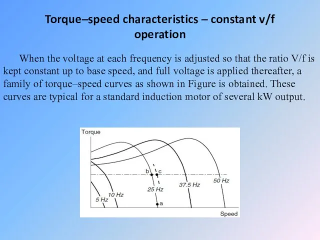
- 17. Torque–speed characteristics – constant v/f operation When the voltage at each frequency is adjusted so that
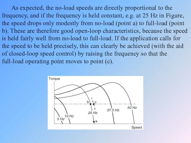
- 18. As expected, the no-load speeds are directly proportional to the frequency, and if the frequency is
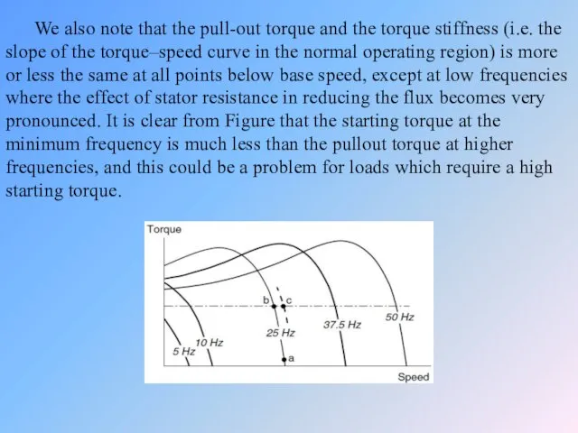
- 19. We also note that the pull-out torque and the torque stiffness (i.e. the slope of the
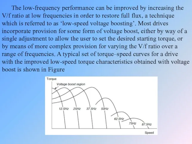
- 20. The low-frequency performance can be improved by increasing the V/f ratio at low frequencies in order
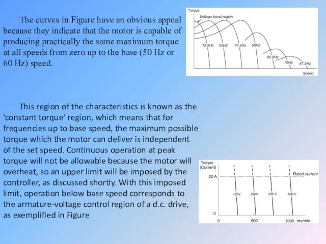
- 21. The curves in Figure have an obvious appeal because they indicate that the motor is capable
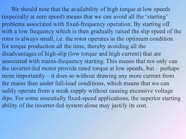
- 22. We should note that the availability of high torque at low speeds (especially at zero speed)
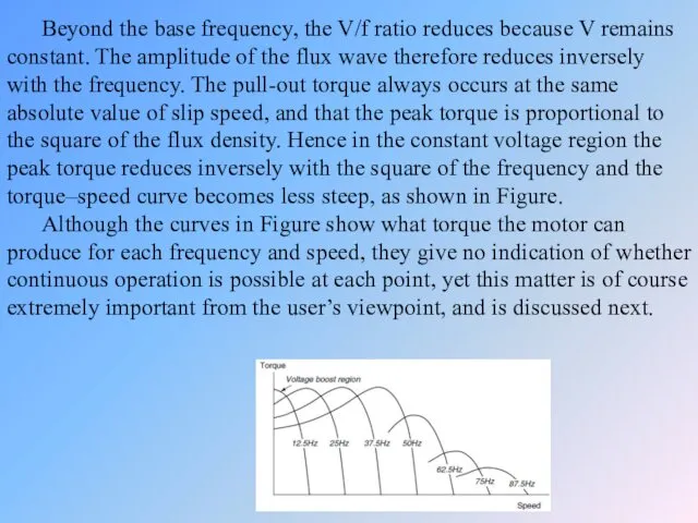
- 23. Beyond the base frequency, the V/f ratio reduces because V remains constant. The amplitude of the
- 24. Modelling the electromechanical energy conversion process The behaviour of the motor was determined primarily by the
- 25. A very important observation in relation to what we are now seeking to do is that
- 26. Hence if we build from the exact transformer circuit, we obtain the induction motor equivalent circuit
- 27. At any given slip, the power delivered to this ‘load’ resistance represents the power crossing the
- 28. Firstly, given the complexity of the spatial and temporal interactions in the induction motor it is
- 29. The key to developing the representation lies in ensuring that the magnitude and phase of the
- 30. In the supply-frequency equivalent circuit, e.g. Figure, the secondary e.m.f. is , rather than , so
- 31. Limitations imposed by the inverter – constant power and constant torque regions The main concern in
- 32. The current limit feature imposes an upper limit on the permissible torque in the region below
- 33. In the region below base speed, the motor can therefore develop any torque up to rated
- 34. At the upper limit of the constant power region, the current limit coincides with the pull-out
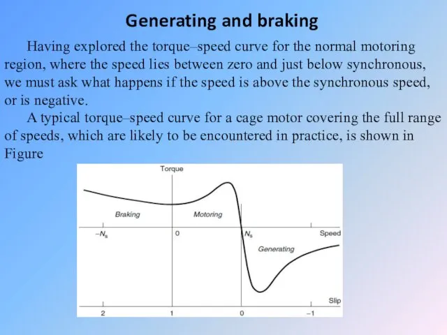
- 35. Generating and braking Having explored the torque–speed curve for the normal motoring region, where the speed
- 40. We can see from Figure that the decisive [diˈsīsiv] factor as far as the direction of
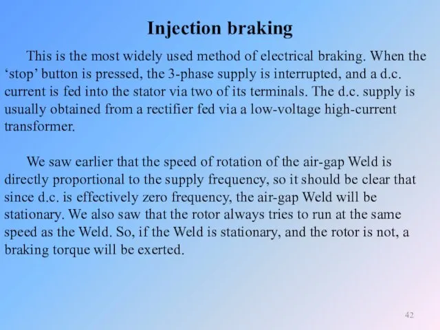
- 42. Injection braking This is the most widely used method of electrical braking. When the ‘stop’ button
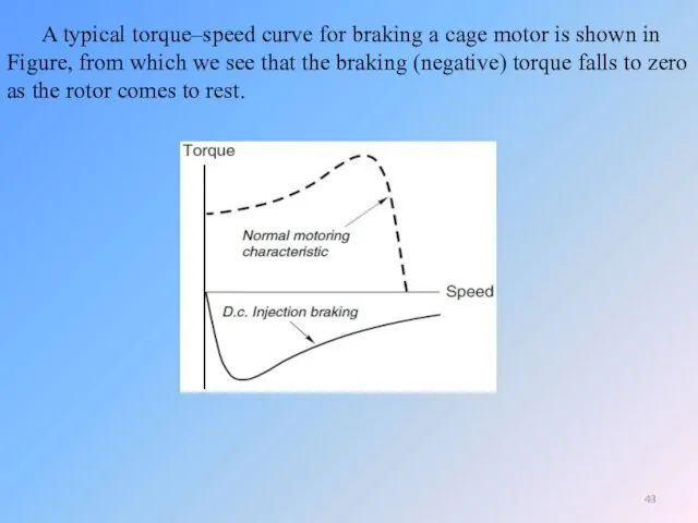
- 43. A typical torque–speed curve for braking a cage motor is shown in Figure, from which we
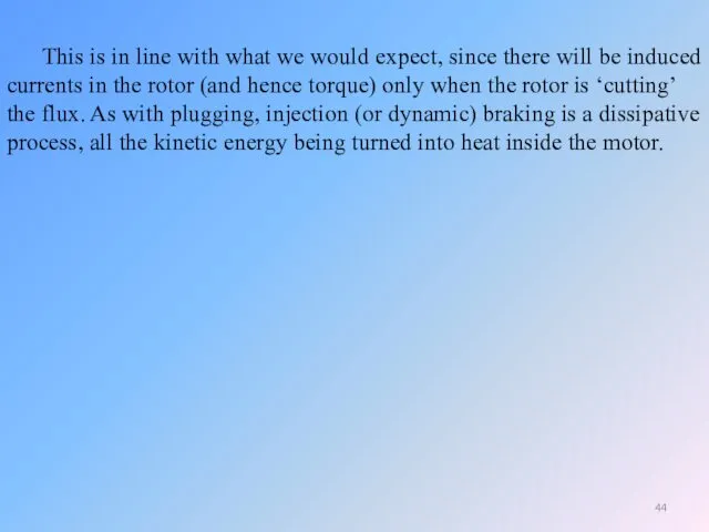
- 44. This is in line with what we would expect, since there will be induced currents in
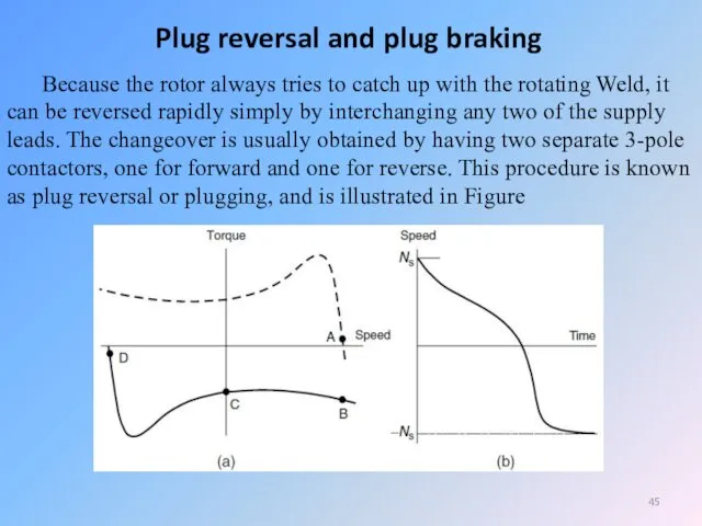
- 45. Plug reversal and plug braking Because the rotor always tries to catch up with the rotating
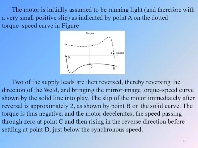
- 46. The motor is initially assumed to be running light (and therefore with a very small positive
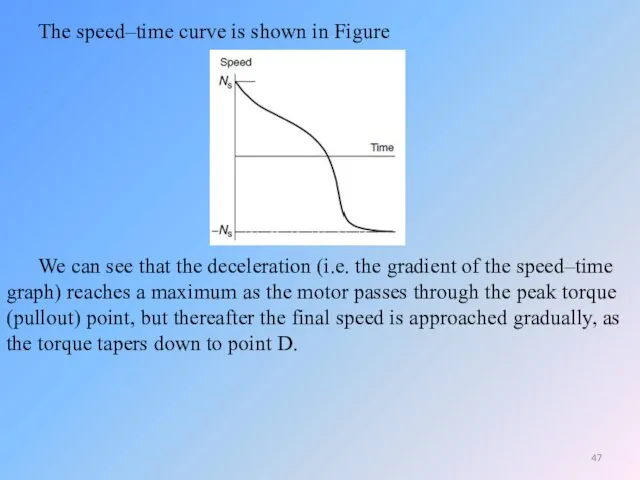
- 47. The speed–time curve is shown in Figure We can see that the deceleration (i.e. the gradient
- 48. Very rapid reversal is possible using plugging; for example a 1 kW motor will typically reverse
- 49. We should note that, whereas, in the regenerative mode (discussed in the previous section) the slip
- 50. Stepping motors Stepping motors are attractive because they can be controlled directly by computers or microcontrollers.
- 51. Performance Features of MOONS' Stepping Motors • Accurate Position Control The number of control pulses defines
- 52. • Forward & Reverse, Pause and Holding Function Motor torque and position control is effective throughout
- 53. Basic Structure and Motor Operation
- 54. A basic stepping motor system is shown in Figure The drive contains the electronic switching circuits,
- 55. This one to one correspondence between pulses and steps is the great attraction of the stepping
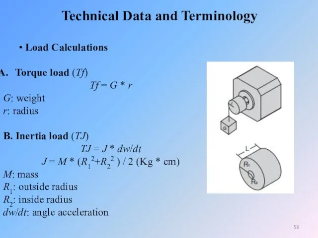
- 56. Technical Data and Terminology • Load Calculations Torque load (Tf) Tf = G * r G:
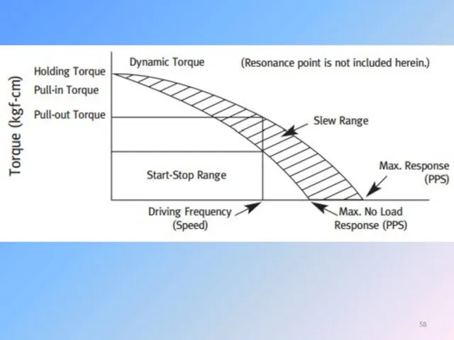
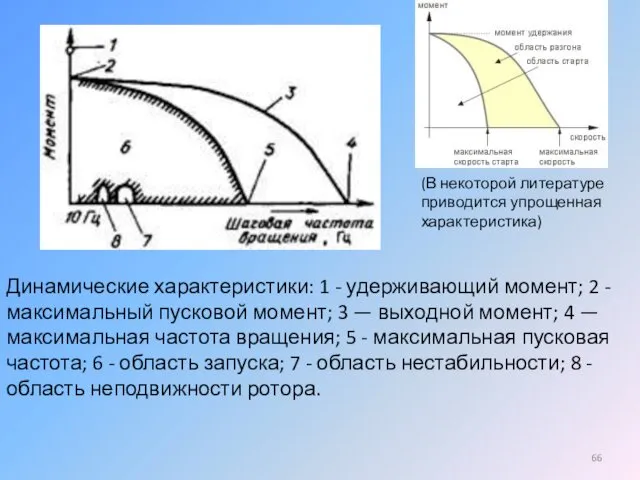
- 57. • Speed-Torque Characteristics The dynamic torque curve is an important aspect of stepping motor’s output performance.
- 59. Борьба с нежелательными явлениями Зазор между роторными и статорными зубцами всегда делается минимальным для увеличения жесткости
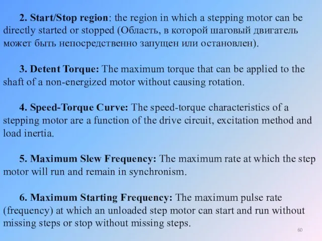
- 60. 2. Start/Stop region: the region in which a stepping motor can be directly started or stopped
- 61. 7. Pull-in Torque: the maximum dynamic torque value that a stepping motor can load directly at
- 62. 10. Accuracy: This is defined as the difference between the theoretical and actual rotor position expressed
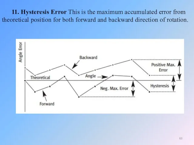
- 63. 11. Hysteresis Error This is the maximum accumulated error from theoretical position for both forward and
- 64. 12. Resonance: A step motor operates on a series of input pulses, each pulse causing the
- 65. Динамические характеристики Динамическими характеристиками называются характеристики двигателя во время движения либо в его начале. Характеристики пускового
- 66. Динамические характеристики: 1 - удерживающий момент; 2 - максимальный пусковой момент; 3 — выходной момент; 4
- 67. Максимальный статический эффект имеет сразу два положения: - Удерживающий. Это максимально допустимый эффект, который теоретически может
- 68. «Мертвые» положения ротора Существует сразу три положения, в которых ротор полностью останавливается: - Положение равновесия. В
- 69. Во всех случаях, когда рассчитывается либо измеряется пусковой момент, необходимо также четко определить схему управления, метод
- 70. Максимальная частота приемистости определяется как максимальная управляющая частота, при которой ненагруженный двигатель может запускаться и останавливаться
- 71. Principle of motor operation The principle on which stepping motors are based is very simple. When
- 72. Before exploring constructional details, it is worth saying a little more about reluctance torque, and its
- 73. The answer is that in the vast majority of electrical machines, from generators in power stations
- 74. As mentioned above, reluctance torque originates in the tendency of an iron bar to align itself
- 75. All the torque is then produced by reluctance action, because with no conductors on the rotor
- 76. Because the two torque-producing mechanisms appear to be radically different, the approaches taken to develop theoretical
- 77. The two most important types of stepping motor are the variable reluctance (VR) type and the
- 78. Motor characteristics Static torque–displacement curves From the previous discussion, it should be clear that the shape
- 79. We now turn to a typical static torque–displacement curve, and look at how it determines motor
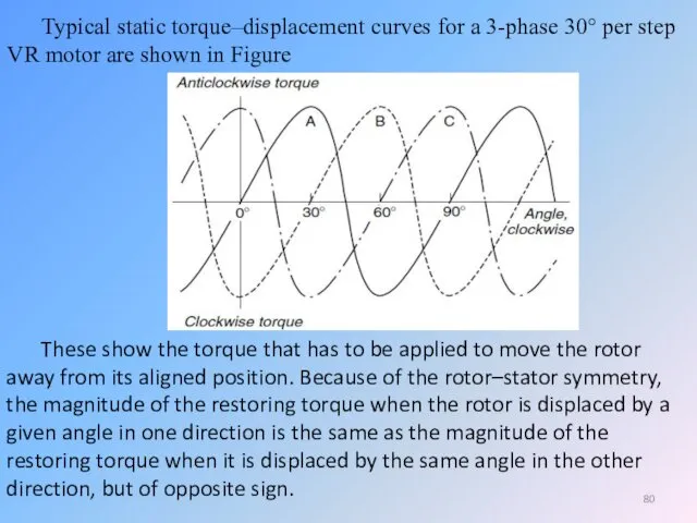
- 80. Typical static torque–displacement curves for a 3-phase 30° per step VR motor are shown in Figure
- 81. There are three curves, one for each of the three phases, and for each curve we
- 82. When only one phase, say A, is energised, the other two phases exert no torque, so
- 83. There are also four unstable equilibrium positions, (at θ = 45°, 135°, 225° and 315°) at
- 84. The characteristic of static (holding) torque - displacement is best explained using an electro-magnet and a
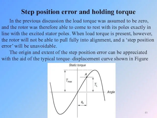
- 85. Step position error and holding torque In the previous discussion the load torque was assumed to
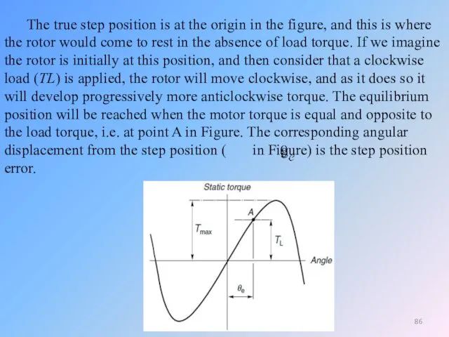
- 86. The true step position is at the origin in the figure, and this is where the
- 87. The existence of a step position error is one of the drawbacks of the stepping motor.
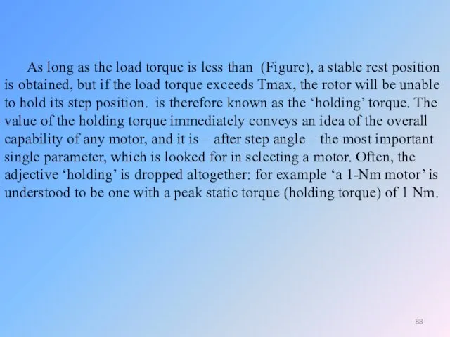
- 88. As long as the load torque is less than (Figure), a stable rest position is obtained,
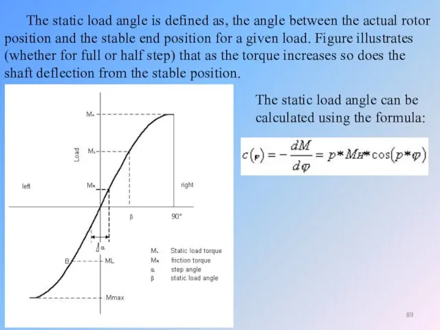
- 89. The static load angle is defined as, the angle between the actual rotor position and the
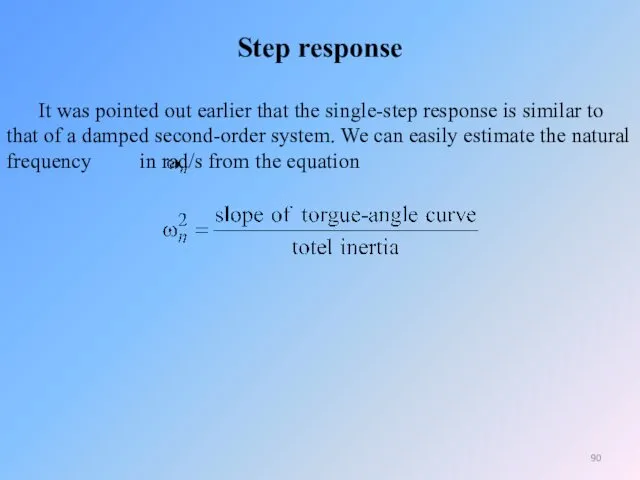
- 90. Step response It was pointed out earlier that the single-step response is similar to that of
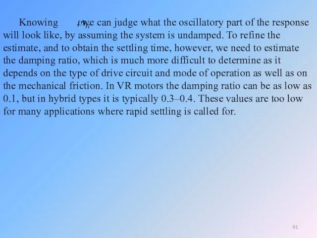
- 91. Knowing , we can judge what the oscillatory part of the response will look like, by
- 93. Скачать презентацию
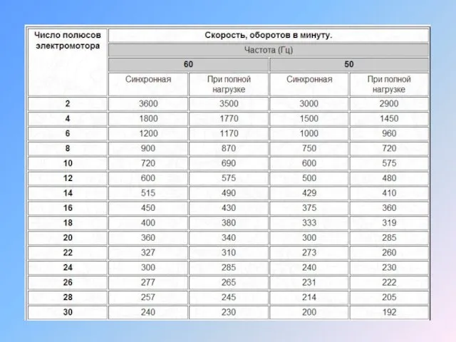
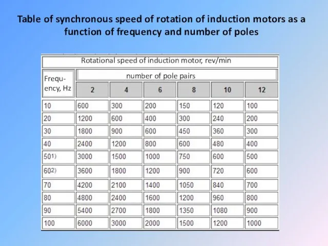
Table of synchronous speed of rotation of induction motors as a
Table of synchronous speed of rotation of induction motors as a
Influence of supply voltage on torque–speed curve
We established earlier that at
Influence of supply voltage on torque–speed curve
We established earlier that at
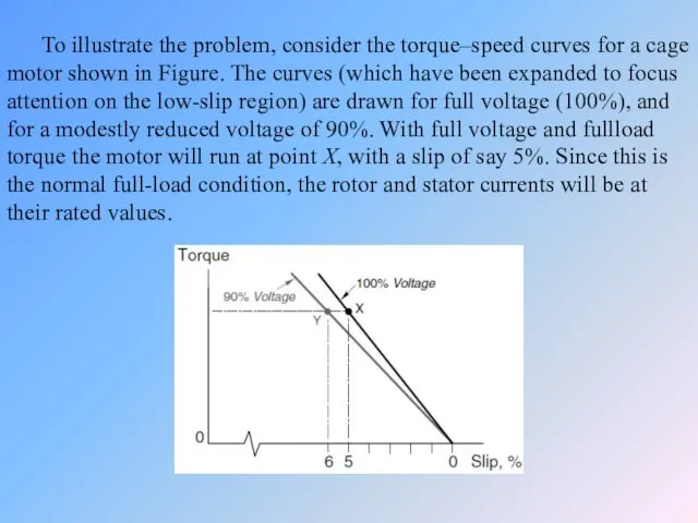
To illustrate the problem, consider the torque–speed curves for a cage
To illustrate the problem, consider the torque–speed curves for a cage
Now suppose that the voltage falls to 90%. The load torque
Now suppose that the voltage falls to 90%. The load torque
The drop in speed from 95% of synchronous to 94% may
The drop in speed from 95% of synchronous to 94% may
Speed control
We have seen that to operate efficiently an induction motor
Speed control
We have seen that to operate efficiently an induction motor
Pole-changing motors
For some applications continuous speed control may be an unnecessary
Pole-changing motors
For some applications continuous speed control may be an unnecessary
It was soon realised that if half of the phase belts
It was soon realised that if half of the phase belts
It was not until the advent of the more sophisticated pole
It was not until the advent of the more sophisticated pole
The beauty of the PAM method is that it is not
The beauty of the PAM method is that it is not
Voltage control of high-resistance cage motors
Where efficiency is not of paramount
Voltage control of high-resistance cage motors
Where efficiency is not of paramount
But if special high-rotor resistance motors are used, the slope of
But if special high-rotor resistance motors are used, the slope of
Voltage control became feasible only when relatively cheap thyristor a.c. voltage
Voltage control became feasible only when relatively cheap thyristor a.c. voltage
Speed control of wound-rotor motors
The fact that the rotor resistance can
Speed control of wound-rotor motors
The fact that the rotor resistance can
Torque–speed characteristics – constant v/f operation
When the voltage at each frequency
Torque–speed characteristics – constant v/f operation
When the voltage at each frequency
As expected, the no-load speeds are directly proportional to the frequency,
As expected, the no-load speeds are directly proportional to the frequency,
We also note that the pull-out torque and the torque stiffness
We also note that the pull-out torque and the torque stiffness
The low-frequency performance can be improved by increasing the V/f ratio
The low-frequency performance can be improved by increasing the V/f ratio
The curves in Figure have an obvious appeal because they indicate
The curves in Figure have an obvious appeal because they indicate
We should note that the availability of high torque at low
We should note that the availability of high torque at low
Beyond the base frequency, the V/f ratio reduces because V remains
Beyond the base frequency, the V/f ratio reduces because V remains
Modelling the electromechanical energy conversion process
The behaviour of the motor was
Modelling the electromechanical energy conversion process
The behaviour of the motor was
A very important observation in relation to what we are now
A very important observation in relation to what we are now
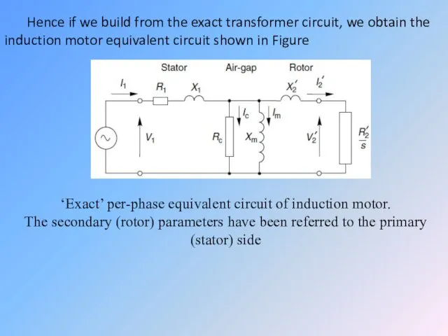
Hence if we build from the exact transformer circuit, we obtain
Hence if we build from the exact transformer circuit, we obtain
At any given slip, the power delivered to this ‘load’ resistance
At any given slip, the power delivered to this ‘load’ resistance
Firstly, given the complexity of the spatial and temporal interactions in
Firstly, given the complexity of the spatial and temporal interactions in
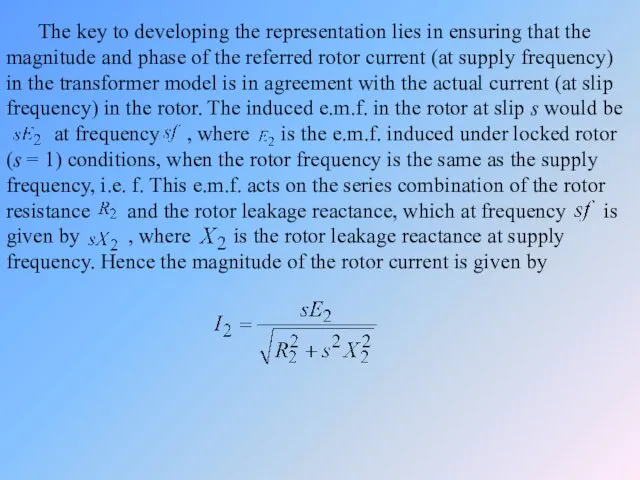
The key to developing the representation lies in ensuring that the
The key to developing the representation lies in ensuring that the
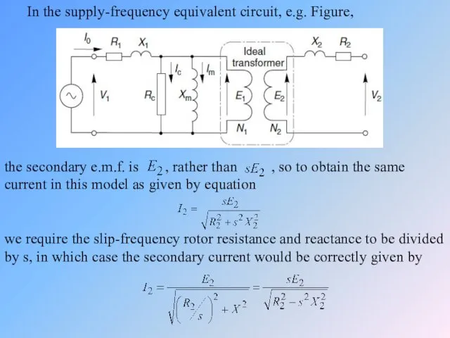
In the supply-frequency equivalent circuit, e.g. Figure,
the secondary e.m.f. is
In the supply-frequency equivalent circuit, e.g. Figure,
the secondary e.m.f. is
Limitations imposed by the inverter – constant power and constant torque
Limitations imposed by the inverter – constant power and constant torque
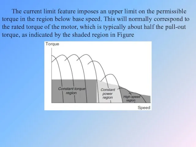
The current limit feature imposes an upper limit on the permissible
The current limit feature imposes an upper limit on the permissible
In the region below base speed, the motor can therefore develop
In the region below base speed, the motor can therefore develop
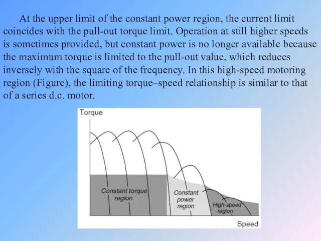
At the upper limit of the constant power region, the current
At the upper limit of the constant power region, the current
Generating and braking
Having explored the torque–speed curve for the normal motoring
Generating and braking
Having explored the torque–speed curve for the normal motoring

![We can see from Figure that the decisive [diˈsīsiv] factor](/_ipx/f_webp&q_80&fit_contain&s_1440x1080/imagesDir/jpg/16902/slide-39.jpg)
We can see from Figure that the decisive [diˈsīsiv] factor as
We can see from Figure that the decisive [diˈsīsiv] factor as
Injection braking
This is the most widely used method of electrical braking.
Injection braking
This is the most widely used method of electrical braking.
A typical torque–speed curve for braking a cage motor is shown
A typical torque–speed curve for braking a cage motor is shown
This is in line with what we would expect, since there
This is in line with what we would expect, since there
Plug reversal and plug braking
Because the rotor always tries to catch
Plug reversal and plug braking
Because the rotor always tries to catch
The motor is initially assumed to be running light (and therefore
The motor is initially assumed to be running light (and therefore
The speed–time curve is shown in Figure
We can see that the
The speed–time curve is shown in Figure
We can see that the
Very rapid reversal is possible using plugging; for example a 1
Very rapid reversal is possible using plugging; for example a 1
We should note that, whereas, in the regenerative mode (discussed in
We should note that, whereas, in the regenerative mode (discussed in
Stepping motors
Stepping motors are attractive because they can be controlled directly
Stepping motors
Stepping motors are attractive because they can be controlled directly
Performance Features of MOONS' Stepping Motors
• Accurate Position Control
The
Performance Features of MOONS' Stepping Motors
• Accurate Position Control
The
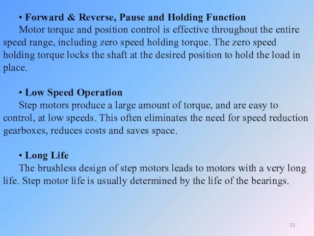
• Forward & Reverse, Pause and Holding Function
Motor torque and
• Forward & Reverse, Pause and Holding Function
Motor torque and
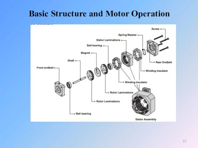
Basic Structure and Motor Operation
Basic Structure and Motor Operation
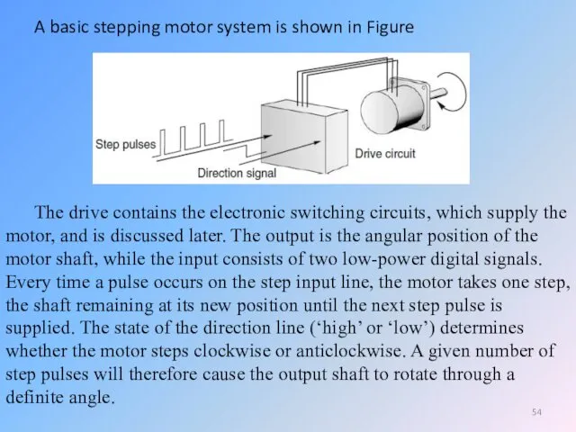
A basic stepping motor system is shown in Figure
The drive contains
A basic stepping motor system is shown in Figure
The drive contains
This one to one correspondence between pulses and steps is the
This one to one correspondence between pulses and steps is the
Technical Data and Terminology
• Load Calculations
Torque load (Tf)
Tf =
Technical Data and Terminology
• Load Calculations
Torque load (Tf)
Tf =
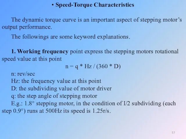
• Speed-Torque Characteristics
The dynamic torque curve is an important aspect of
• Speed-Torque Characteristics
The dynamic torque curve is an important aspect of

Борьба с нежелательными явлениями
Зазор между роторными и статорными зубцами всегда
Борьба с нежелательными явлениями
Зазор между роторными и статорными зубцами всегда
2. Start/Stop region: the region in which a stepping motor can
2. Start/Stop region: the region in which a stepping motor can
7. Pull-in Torque: the maximum dynamic torque value that a stepping
7. Pull-in Torque: the maximum dynamic torque value that a stepping
10. Accuracy: This is defined as the difference between the theoretical
10. Accuracy: This is defined as the difference between the theoretical
11. Hysteresis Error This is the maximum accumulated error from theoretical
11. Hysteresis Error This is the maximum accumulated error from theoretical
12. Resonance: A step motor operates on a series of input
12. Resonance: A step motor operates on a series of input

Динамические характеристики
Динамическими характеристиками называются характеристики двигателя во время движения либо в
Динамические характеристики
Динамическими характеристиками называются характеристики двигателя во время движения либо в
Динамические характеристики: 1 - удерживающий момент; 2 - максимальный пусковой момент;
Динамические характеристики: 1 - удерживающий момент; 2 - максимальный пусковой момент;

Максимальный статический эффект имеет сразу два положения:
- Удерживающий. Это максимально
Максимальный статический эффект имеет сразу два положения:
- Удерживающий. Это максимально

«Мертвые» положения ротора
Существует сразу три положения, в которых ротор полностью
«Мертвые» положения ротора
Существует сразу три положения, в которых ротор полностью

Во всех случаях, когда рассчитывается либо измеряется пусковой момент, необходимо также
Во всех случаях, когда рассчитывается либо измеряется пусковой момент, необходимо также

Максимальная частота приемистости определяется как максимальная управляющая частота, при которой ненагруженный
Максимальная частота приемистости определяется как максимальная управляющая частота, при которой ненагруженный
Principle of motor operation
The principle on which stepping motors are based
Principle of motor operation
The principle on which stepping motors are based
Before exploring constructional details, it is worth saying a little more
Before exploring constructional details, it is worth saying a little more
The answer is that in the vast majority of electrical machines,
The answer is that in the vast majority of electrical machines,
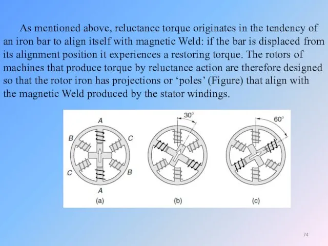
As mentioned above, reluctance torque originates in the tendency of an
As mentioned above, reluctance torque originates in the tendency of an
All the torque is then produced by reluctance action, because with
All the torque is then produced by reluctance action, because with
Because the two torque-producing mechanisms appear to be radically different, the
Because the two torque-producing mechanisms appear to be radically different, the
The two most important types of stepping motor are the variable
The two most important types of stepping motor are the variable
Motor characteristics
Static torque–displacement curves
From the previous discussion, it should be clear
Motor characteristics
Static torque–displacement curves
From the previous discussion, it should be clear
We now turn to a typical static torque–displacement curve, and look
We now turn to a typical static torque–displacement curve, and look
Typical static torque–displacement curves for a 3-phase 30° per step VR
Typical static torque–displacement curves for a 3-phase 30° per step VR
There are three curves, one for each of the three phases,
There are three curves, one for each of the three phases,
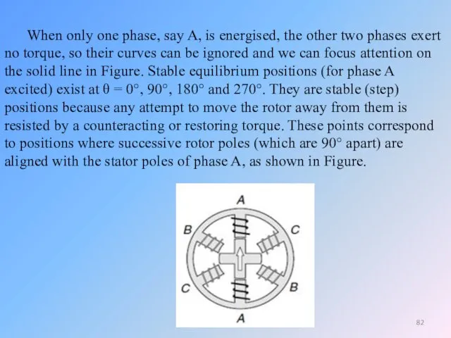
When only one phase, say A, is energised, the other two
When only one phase, say A, is energised, the other two
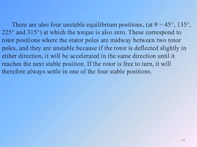
There are also four unstable equilibrium positions, (at θ = 45°,
There are also four unstable equilibrium positions, (at θ = 45°,
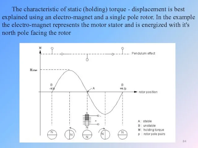
The characteristic of static (holding) torque - displacement is best explained
The characteristic of static (holding) torque - displacement is best explained
Step position error and holding torque
In the previous discussion the load
Step position error and holding torque
In the previous discussion the load
The true step position is at the origin in the figure,
The true step position is at the origin in the figure,
The existence of a step position error is one of the
The existence of a step position error is one of the
As long as the load torque is less than (Figure), a
As long as the load torque is less than (Figure), a
The static load angle is defined as, the angle between the
The static load angle is defined as, the angle between the
Step response
It was pointed out earlier that the single-step response is
Step response
It was pointed out earlier that the single-step response is
Knowing , we can judge what the oscillatory part of the
Knowing , we can judge what the oscillatory part of the
 Электрооборудование автомобилей. Контрольно-измерительные приборы. (Урок 10)
 Организация дистанционной формы обучения физике 7-9 классов обучащихся с ОВЗ
 Электор жабдықтау жүиесі,оталдыру және іске қосу жүиесі
 Физика, математика
 Устройство и принцип действия тепловых машин
 Законы сохранения в механике
 Понятие Биологическое действие радиации
 Деление ядер урана. Цепная ядерная реакция
 Классификация способов обработки материалов потоками излучения
 Магнитные свойства вещества. 10 класс
 Реактивное движение. Физический диктант
 презентация и методическое описание к уроку Звук
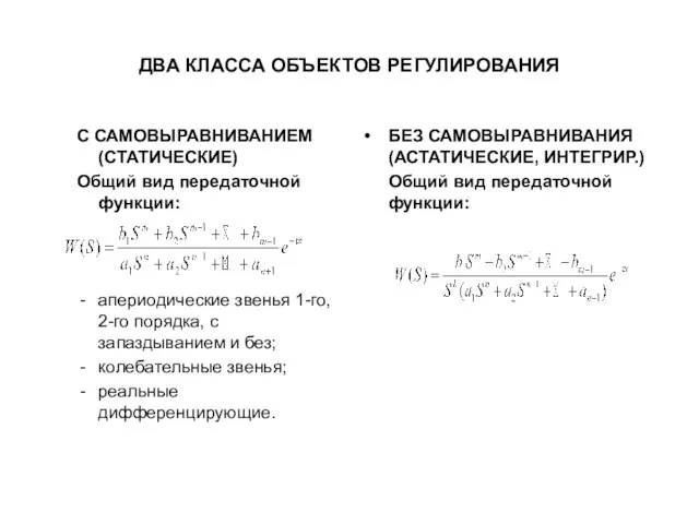 Два класса объектов регулирования
 Презентация к уроку физики по теме Сила тяжести.Вес тела
 Трансформаторы. Виды трансформаторов
 Воздухоплавание. Первый воздушный полёт
 Гидравлический домкрат в быту
 Динамика вращательного движения
 Гармонические колебания. Свободные колебания. Вынужденные колебания
 Изобретение электричества. История, применение, получение
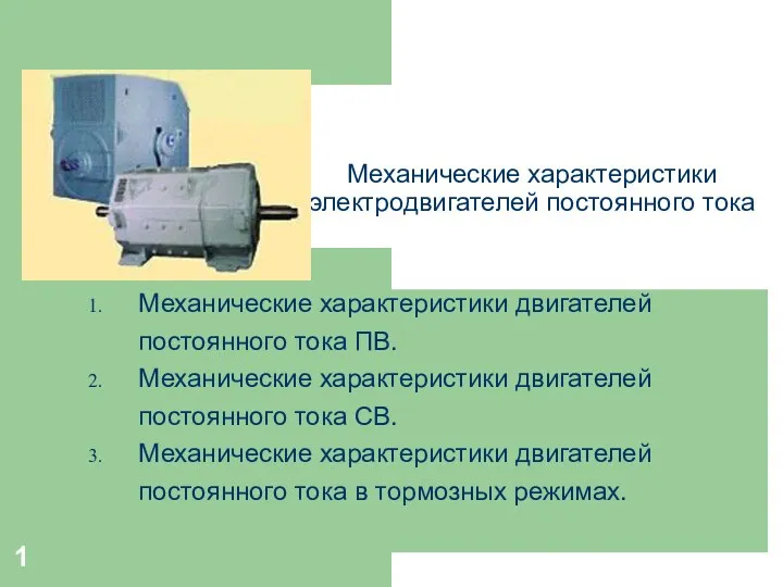 Механические характеристики электродвигателей постоянного тока
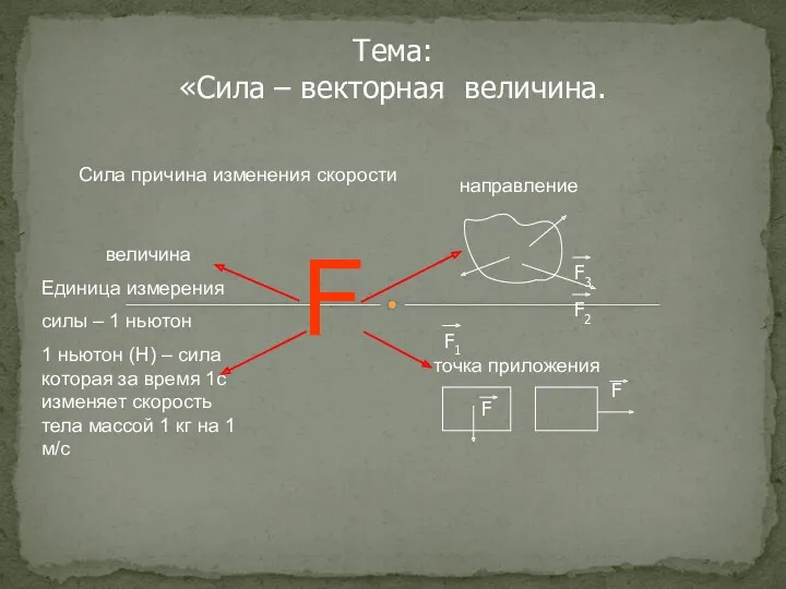 Сила – векторная величина
 Радиоволны и радио
 История создания швейной машины. Бытовая швейная машина
 Электромагнитные зондирования (ВЭЗ, ДЭЗ, ВЭЗ-ВП, ЧЗ, ЗС, МТЗ)
 Радиациялық сәулелену
 Кинематические характеристики движения точки
 открытый урок по теме Термодинамическая система. Внутренняя энергия