Accounting applications on introduction computer to Microsoft Excel презентация

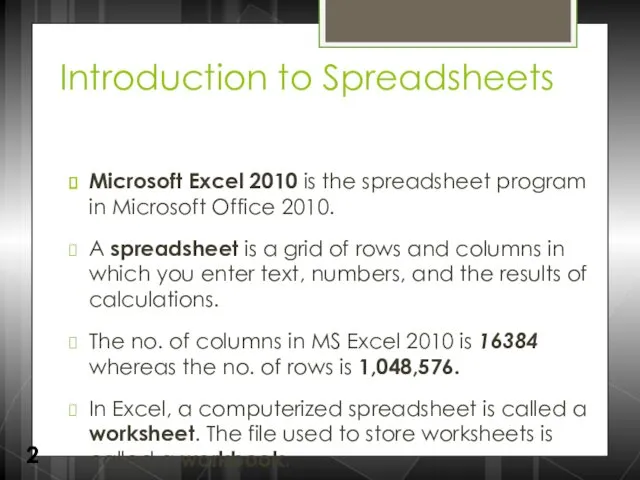
Introduction to Spreadsheets
Microsoft Excel 2010 is the spreadsheet program in Microsoft Office 2010.
A spreadsheet is a grid of rows and columns in which you enter text, numbers, and the results of calculations.
The no. of columns in MS Excel 2010 is 16384 whereas the no. of rows is 1,048,576.
In Excel, a computerized spreadsheet is called a worksheet. The file used to store worksheets is called a workbook.

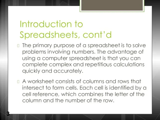
Introduction to Spreadsheets, cont’d
The primary purpose of a spreadsheet is to solve problems involving numbers. The advantage of using a computer spreadsheet is that you can complete complex and repetitious calculations quickly and accurately.
A worksheet consists of columns and rows that intersect to form cells. Each cell is identified by a cell reference, which combines the letter of the column and the number of the row.

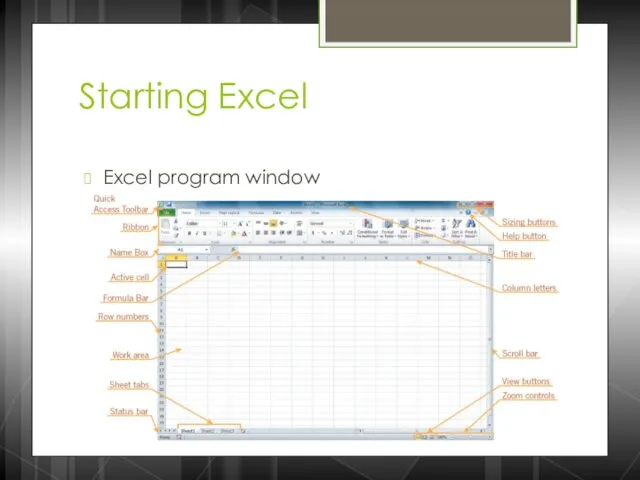
Starting Excel
Excel program window

Saving a Workbook
The Save command saves an existing workbook, using its current name and save location.
The Save As command lets you save a workbook with a new name or to a new location.

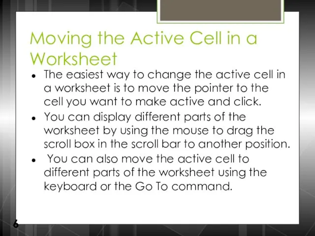
Moving the Active Cell in a Worksheet
The easiest way to change the active cell in a worksheet is to move the pointer to the cell you want to make active and click.
You can display different parts of the worksheet by using the mouse to drag the scroll box in the scroll bar to another position.
You can also move the active cell to different parts of the worksheet using the keyboard or the Go To command.

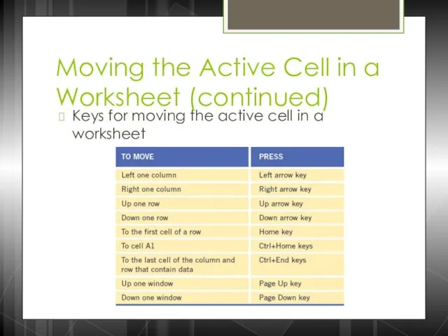
Moving the Active Cell in a Worksheet (continued)
Keys for moving the active cell in a worksheet

Selecting a Group of Cells
A group of selected cells is called a range. The range is identified by its range reference, for example, A3:C5.
In an adjacent range, all cells touch each other and form a rectangle.
To select an adjacent range, click the cell in a corner of the range, drag the pointer to the cell in the opposite corner of the range, and release the mouse button.

Selecting a Group of Cells (continued)
A nonadjacent range includes two or more adjacent ranges and selected cells.
To select a nonadjacent range, select the first adjacent range or cell, press the Ctrl key as you select the other cells or ranges you want to include, and then release the Ctrl key and the mouse button.

Entering Data in a Cell
Worksheet cells can contain text, numbers, or formulas.
Text is any combination of letters and numbers and symbols.
Numbers are values, dates, or times.
Formulas are equations that calculate a value.
You enter data in the active cell.

Data Entry
The simplest way to enter data is to click a cell and type a value. This method works very well when you’re entering a few pieces of data, but it is less than ideal when you’re entering long sequences or series of values.
Example:
If you want to create a worksheet containing the sales revenues for the companies branches in Qena, Luxor, and Aswan for the first quarter in 2014. To record theses numbers you need to create a worksheet tracking each branch monthly sales.

Data Entry
Repeatedly entering the sequence January, February, March, and so on can be handled by copying and pasting the first occurrence of the sequence, but there’s an easier way to do it: use AutoFill.
With AutoFill, you enter the first element in a recognized series, click and hold the mouse button down on the fill handle at the lower-right corner of the cell, and drag the fill handle until the series extends far enough to accommodate your data.
Using a similar tool, FillSeries, you can enter two values in a series and use the fill handle to extend the series in your worksheet. For example, if you want to create a series starting at 2 and increasing by 2, you can put 2 in the first cell and 4 in the second cell, select both cells, and then use the fill handle to extend the series to your desired end value.

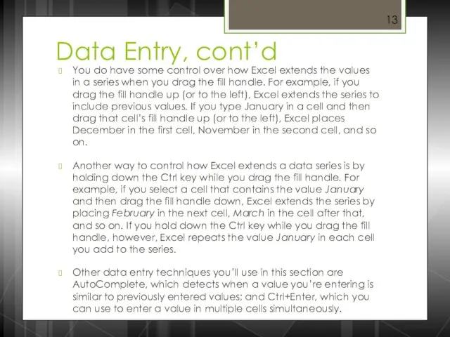
Data Entry, cont’d
You do have some control over how Excel extends the values in a series when you drag the fill handle. For example, if you drag the fill handle up (or to the left), Excel extends the series to include previous values. If you type January in a cell and then drag that cell’s fill handle up (or to the left), Excel places December in the first cell, November in the second cell, and so on.
Another way to control how Excel extends a data series is by holding down the Ctrl key while you drag the fill handle. For example, if you select a cell that contains the value January and then drag the fill handle down, Excel extends the series by placing February in the next cell, March in the cell after that, and so on. If you hold down the Ctrl key while you drag the fill handle, however, Excel repeats the value January in each cell you add to the series.
Other data entry techniques you’ll use in this section are AutoComplete, which detects when a value you’re entering is similar to previously entered values; and Ctrl+Enter, which you can use to enter a value in multiple cells simultaneously.

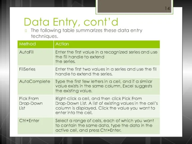
Data Entry, cont’d
The following table summarizes these data entry techniques.

Changing Data in a Cell
You can edit, replace, or clear data.
You can edit cell data in the Formula Bar or in the cell. The contents of the active cell always appear in the Formula Bar.
To replace cell data, select the cell, type new data, and press the Enter button on the Formula Bar or the Enter key or the keyboard.

Searching for Data
The Find command locates data in a worksheet, which is particularly helpful when a worksheet contains a large amount of data. You can use the Find command to locate words or parts of words.
The Replace command is an extension of the Find command. Replacing data substitutes new data for the data that the Find command locates.

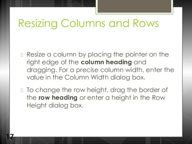
Resizing Columns and Rows
Resize a column by placing the pointer on the right edge of the column heading and dragging. For a precise column width, enter the value in the Column Width dialog box.
To change the row height, drag the border of the row heading or enter a height in the Row Height dialog box.

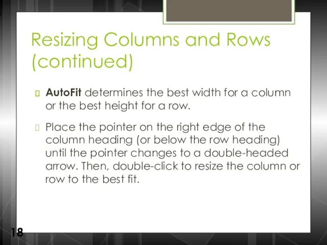
Resizing Columns and Rows (continued)
AutoFit determines the best width for a column or the best height for a row.
Place the pointer on the right edge of the column heading (or below the row heading) until the pointer changes to a double-headed arrow. Then, double-click to resize the column or row to the best fit.

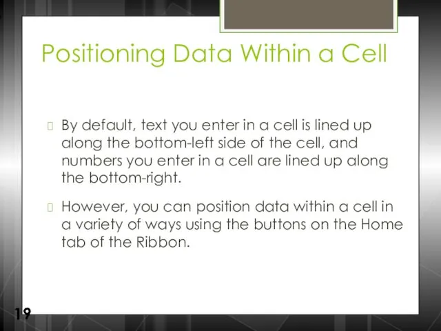
Positioning Data Within a Cell
By default, text you enter in a cell is lined up along the bottom-left side of the cell, and numbers you enter in a cell are lined up along the bottom-right.
However, you can position data within a cell in a variety of ways using the buttons on the Home tab of the Ribbon.

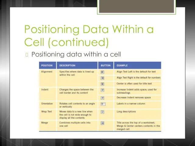
Positioning Data Within a Cell (continued)
Positioning data within a cell

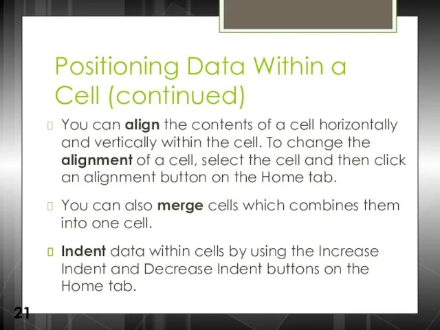
Positioning Data Within a Cell (continued)
You can align the contents of a cell horizontally and vertically within the cell. To change the alignment of a cell, select the cell and then click an alignment button on the Home tab.
You can also merge cells which combines them into one cell.
Indent data within cells by using the Increase Indent and Decrease Indent buttons on the Home tab.

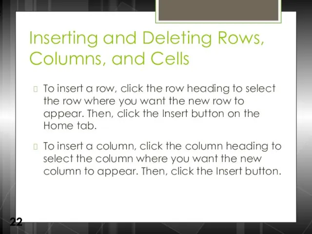
Inserting and Deleting Rows, Columns, and Cells
To insert a row, click the row heading to select the row where you want the new row to appear. Then, click the Insert button on the Home tab.
To insert a column, click the column heading to select the column where you want the new column to appear. Then, click the Insert button.

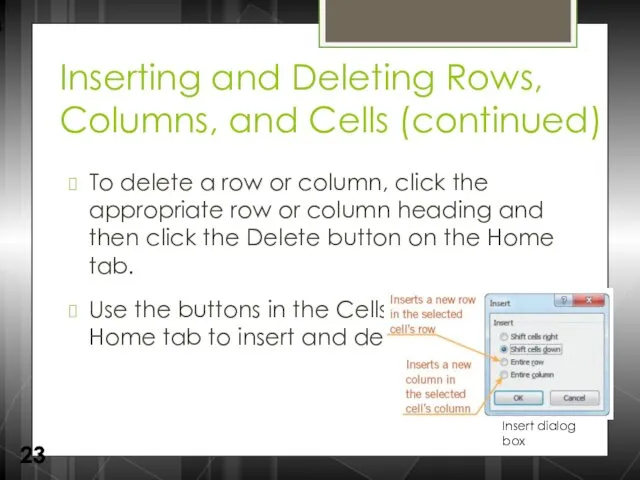
Inserting and Deleting Rows, Columns, and Cells (continued)
To delete a row or column, click the appropriate row or column heading and then click the Delete button on the Home tab.
Use the buttons in the Cells group on the Home tab to insert and delete cells.
Insert dialog box

Freezing Panes in a Worksheet
You can view two parts of a worksheet at once by freezing panes.
When you freeze panes, you select which rows and/or columns of the worksheet remain visible on the screen as the rest of the worksheet scrolls.

Splitting a Worksheet Window
Splitting divides the worksheet window into two or four panes that you can scroll independently.
This enables you to see different parts of a worksheet at the same time.

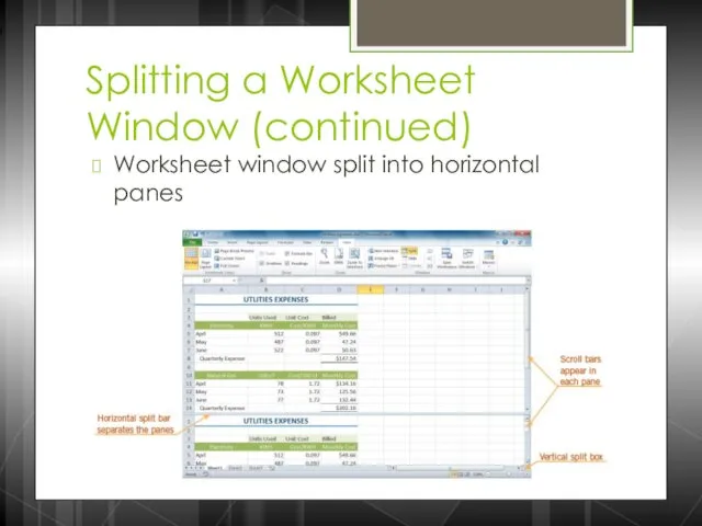
Splitting a Worksheet Window (continued)
Worksheet window split into horizontal panes

Preparing a Worksheet for Printing
So far, you have worked in Normal view, which is the best view for entering and formatting data in a worksheet.
Page Layout view shows how the worksheet will appear on paper, which is helpful when you prepare a worksheet for printing.
The margin is the blank space around the top, bottom, left, and right sides of a page.

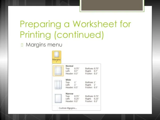
Preparing a Worksheet for Printing (continued)
Margins menu

Preparing a Worksheet for Printing (continued)
By default, Excel is set to print pages in portrait orientation. Worksheets printed in portrait orientation are longer than they are wide. In contrast, worksheets printed in landscape orientation are wider than they are long.
The print area consists of the cells and ranges designated for printing.

Preparing a Worksheet for Printing (continued)
Excel inserts an automatic page break whenever it runs out of room on a page. You can also insert a manual page break to start a new page.
The simplest way to adjust page breaks is in Page Break Preview. On the status bar, click the Page Break Preview button to switch to this view.

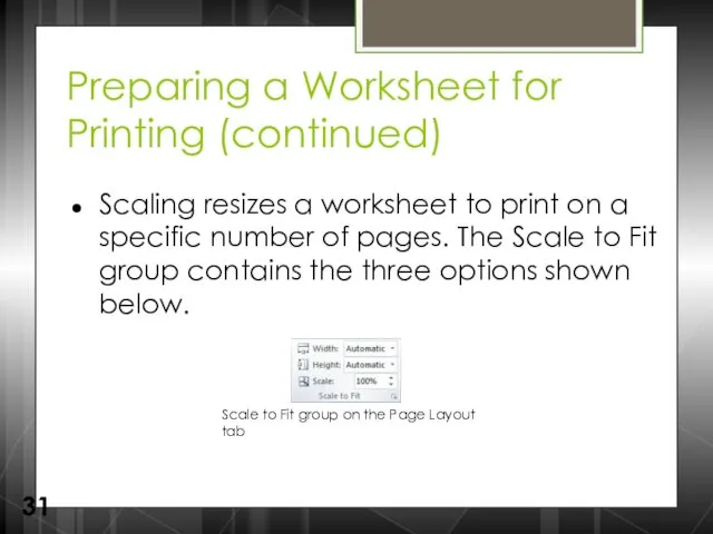
Preparing a Worksheet for Printing (continued)
Scaling resizes a worksheet to print on a specific number of pages. The Scale to Fit group contains the three options shown below.
Scale to Fit group on the Page Layout tab

Preparing a Worksheet for Printing (continued)
By default, gridlines, row numbers, and column letters appear in the worksheet but not on the printed page. You can choose to show or hide gridlines and headings in a worksheet or on the printed page.
Print titles are designated rows and/or columns in a worksheet that are printed on each page.

Comparing Relative, Absolute, and Mixed Cell References
A relative cell reference adjusts to its new location when copied or moved to another cell.
Absolute cell references do not change when copied or moved to a new cell.
Cell references that contain both relative and absolute references are called mixed cell references.
References preceded by a dollar sign do not change.