- Basics of time series forecasting. Lecture 9

Содержание
- 2. LECTURE 9 BASICS OF TIME SERIES FORECASTING Saidgozi Saydumarov Sherzodbek Safarov QM Module Leaders ssaydumarov@wiut.uz s.safarov@wiut.uz
- 3. Lecture outline: to estimate the change of a value over time and graph the dynamics of
- 4. Components of time series graph Trend – the overall pattern of changes in a specific value
- 5. Additive vs Multiplicative Model Additive model Multiplicative model
- 6. Case 1: quarterly computer sales
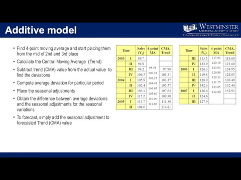
- 7. Additive model Find 4-point moving average and start placing them from the mid of 2nd and
- 8. Additive model
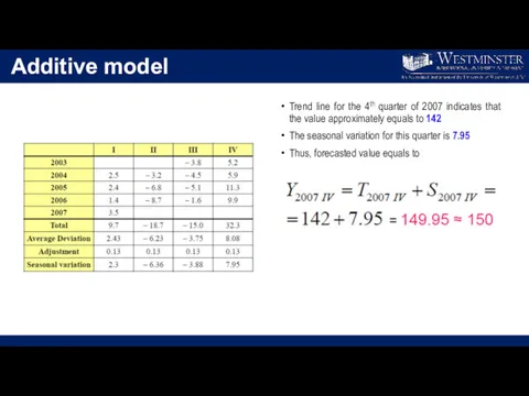
- 9. Additive model Trend line for the 4th quarter of 2007 indicates that the value approximately equals
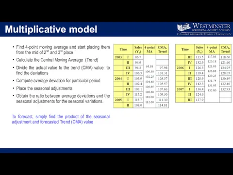
- 10. Multiplicative model Find 4-point moving average and start placing them from the mid of 2nd and
- 11. Multiplicative model
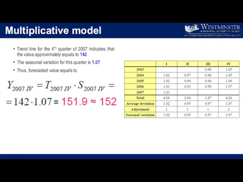
- 12. Multiplicative model Trend line for the 4th quarter of 2007 indicates that the value approximately equals
- 13. Concluding remarks Today, you learned Graphical display of the change of a value over time Time
- 15. Скачать презентацию
LECTURE 9
BASICS OF TIME SERIES FORECASTING
Saidgozi Saydumarov
Sherzodbek Safarov
QM Module Leaders
ssaydumarov@wiut.uz
s.safarov@wiut.uz
Office
LECTURE 9
BASICS OF TIME SERIES FORECASTING
Saidgozi Saydumarov
Sherzodbek Safarov
QM Module Leaders
ssaydumarov@wiut.uz
s.safarov@wiut.uz
Office
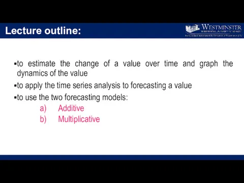
Lecture outline:
to estimate the change of a value over time and
Lecture outline:
to estimate the change of a value over time and
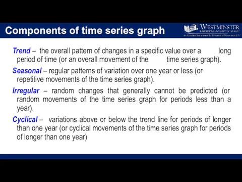
Components of time series graph
Trend – the overall pattern of changes
Components of time series graph
Trend – the overall pattern of changes
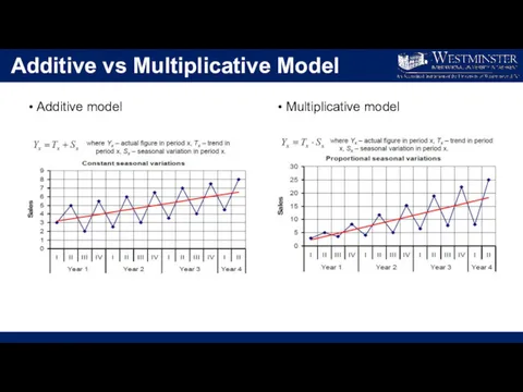
Additive vs Multiplicative Model
Additive model
Multiplicative model
Additive vs Multiplicative Model
Additive model
Multiplicative model
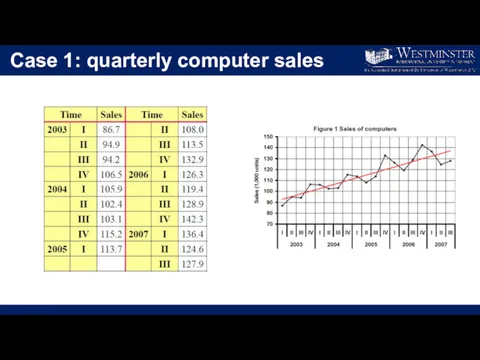
Case 1: quarterly computer sales
Case 1: quarterly computer sales
Additive model
Find 4-point moving average and start placing them from the
Additive model
Find 4-point moving average and start placing them from the
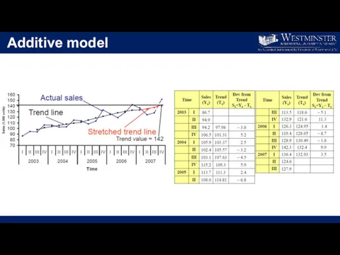
Additive model
Additive model
Additive model
Trend line for the 4th quarter of 2007 indicates that
Additive model
Trend line for the 4th quarter of 2007 indicates that
Multiplicative model
Find 4-point moving average and start placing them from the
Multiplicative model
Find 4-point moving average and start placing them from the
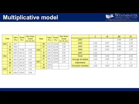
Multiplicative model
Multiplicative model
Multiplicative model
Trend line for the 4th quarter of 2007 indicates that
Multiplicative model
Trend line for the 4th quarter of 2007 indicates that
Concluding remarks
Today, you learned
Graphical display of the change of a value
Concluding remarks
Today, you learned
Graphical display of the change of a value
 Алгоритмы
 Глобальные сети
 Путешествие в страну Информатика. 8 класс
 CISCO CCIE Program
 Моделирование корреляционных зависимостей
 Интернет-зависимость
 Настройка коммутаторов Cisco
 Конвергентные и цифровые технологии
 Деловая графика в электронных таблицах.
 Инженерия программного обеспечения. Введение (модуль 1)
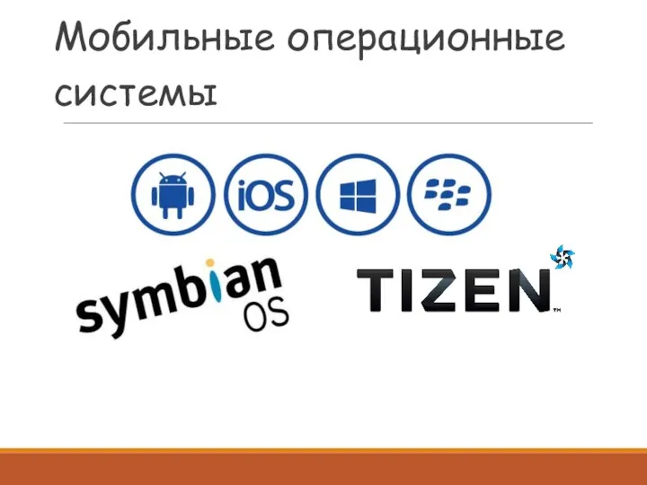 Мобильные операционные системы
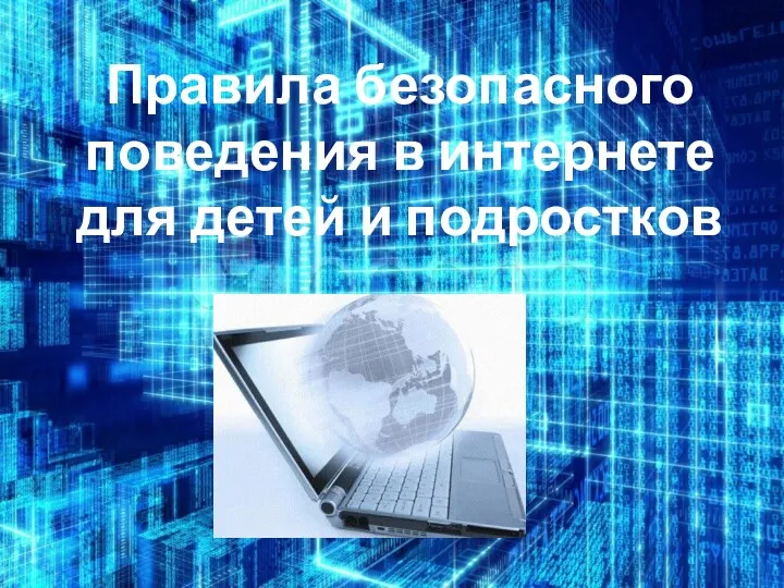 Рекомендации психолога
 Многоуровневые ИВС и эталонная модель взаимосвязи открытых систем. Занятие 05, 06
 Компьютерные объекты
 История развития компьютерной техники. 8 класс
 Завдання: Написати програму, яка переводить числа з арабської системи в римську
 OSINT(Open Source Intelligency)
 Урок по теме Работа со шрифтами. Форматирование текста. 8 класс.
 Регистрация в WealTcom
 Презентация Перевод чисел между системами счисления, основания которых являются степенями числа 2 10 класс
 Информационно-логические основы ЭВМ
 Тораптық утелиттердің жұмысын оқып үйрену
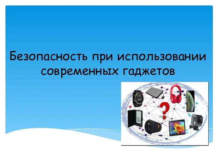 Безопасность при использовании современных гаджетов
 Тестирование мобильных приложений
 Текстові і графічні обʼєкти на слайдах. Урок 30
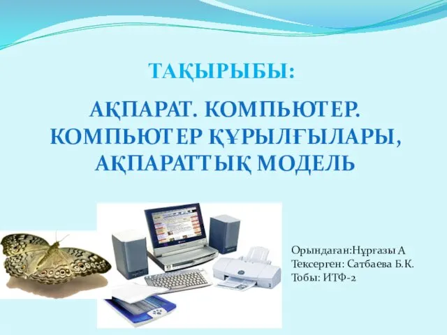 Ақпарат. Компьютер. Компьютер құрылғылары,ақпараттық модель
 Первый канал
 Первоначальные сведения о мониторах