- Game-Theoretic Methods in Machine Learning

Содержание
- 2. From Cliques to Equilibria Dominant-Set Clustering and Its Applications
- 3. The “Classical” Clustering Problem Given: a set of n “objects” an n × n matrix A
- 4. Applications Clustering problems abound in many areas of computer science and engineering. A short list of
- 5. What is a Cluster? No universally accepted (formal) definition of a “cluster” but, informally, a cluster
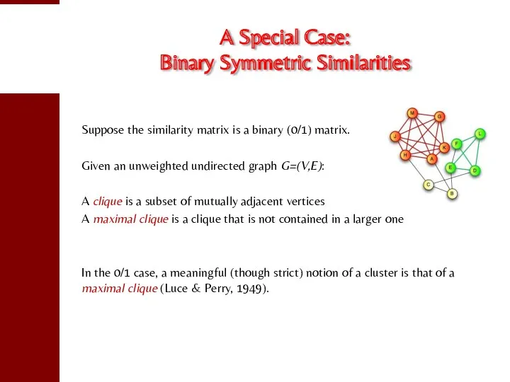
- 6. A Special Case: Binary Symmetric Similarities Suppose the similarity matrix is a binary (0/1) matrix. Given
- 7. Advantages of the New Approach No need to know the number of clusters in advance (since
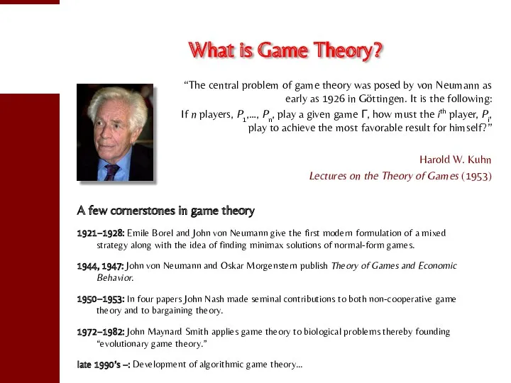
- 8. What is Game Theory? A few cornerstones in game theory 1921−1928: Emile Borel and John von
- 9. “Solving” a Game Nash equilibrium!
- 10. Basics of (Two-Player, Symmetric) Game Theory Assume: a (symmetric) game between two players complete knowledge a
- 11. Nash Equilibria Let A be an arbitrary payoff matrix: aij is the payoff obtained by playing
- 12. Evolution and the Theory of Games “We repeat most emphatically that our theory is thoroughly static.
- 13. Evolutionary Games and ESS’s Assumptions: A large population of individuals belonging to the same species which
- 14. ESS’s as Clusters We claim that ESS’s abstract well the main characteristics of a cluster: Internal
- 15. Basic Definitions Let S ⊆ V be a non-empty subset of vertices, and i∈S. The (average)
- 16. Assigning Weights to Vertices Let S ⊆ V be a non-empty subset of vertices, and i∈S.
- 17. Interpretation Intuitively, wS(i) gives us a measure of the overall (relative) similarity between vertex i and
- 18. Dominant Sets Definition (Pavan and Pelillo, 2003, 2007). A non-empty subset of vertices S ⊆ V
- 19. The Clustering Game Consider the following “clustering game.” Assume a preexisting set of objects O and
- 20. Dominant Sets are ESS’s Theorem (Torsello, Rota Bulò and Pelillo, 2006). Evolutionary stable strategies of the
- 21. Special Case: Symmetric Affinities Given a symmetric real-valued matrix A (with null diagonal), consider the following
- 22. Replicator Dynamics Let xi(t) the population share playing pure strategy i at time t. The state
- 23. Doubly Symmetric Games In a doubly symmetric (or partnership) game, the payoff matrix A is symmetric
- 24. Discrete-time Replicator Dynamics A well-known discretization of replicator dynamics, which assumes non-overlapping generations, is the following
- 25. A Toy Example
- 26. Measuring the Degree of Cluster Membership The components of the converged vector give us a measure
- 27. Application to Image Segmentation An image is represented as an edge-weighted undirected graph, where vertices correspond
- 28. Experimental Setup
- 29. Intensity Segmentation Results Dominant sets Ncut
- 30. Intensity Segmentation Results Dominant sets Ncut
- 31. Results on the Berkeley Dataset Dominant sets Ncut
- 32. Color Segmentation Results Original image Dominant sets Ncut
- 33. Dominant sets Ncut Results on the Berkeley Dataset
- 34. Texture Segmentation Results Dominant sets
- 35. Texture Segmentation Results NCut
- 37. F-formations “Whenever two or more individuals in close proximity orient their bodies in such a way
- 38. System Architecture Frustrum of visual attention A person in a scene is described by his/her position
- 39. Results
- 40. Qualitative results on the CoffeeBreak dataset compared with the state of the art HFF. Yellow =
- 41. Bioinformatics Identification of protein binding sites (Zauhar and Bruist, 2005) Clustering gene expression profiles (Li et
- 42. Extensions
- 43. First idea: run replicator dynamics from different starting points in the simplex. Problem: computationally expensive and
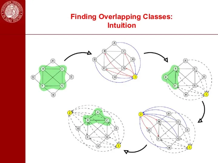
- 44. Finding Overlapping Classes: Intuition
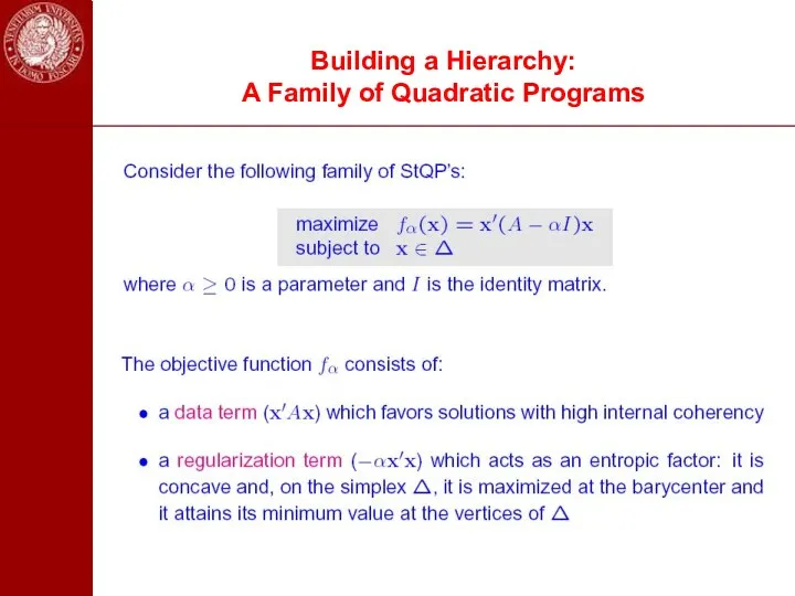
- 45. Building a Hierarchy: A Family of Quadratic Programs
- 46. The effects of α
- 47. The Landscape of fα
- 48. Sketch of the Hierarchical Clustering Algorithm
- 49. Dealing with High-Order Similarities A (weighted) hypergraph is a triplet H = (V, E, w), where
- 50. The Hypergraph Clustering Game Given a weighted k-graph representing an instance of a hypergraph clustering problem,
- 51. ESS’s and Polynomial Optimization
- 52. Baum-Eagon Inequality
- 53. An exampe: Line Clustering
- 54. In a nutshell… The game-theoretic/dominant-set approach: makes no assumption on the structure of the affinity matrix,
- 55. References S. Rota Bulò and M. Pelillo. Dominant-set clustering: A review. Europ. J. Oper. Res. (2017)
- 56. Hume-Nash Machines Context-Aware Models of Learning and Recognition
- 57. Machine learning: The standard paradigm From: Duda, Hart and Stork, Pattern Classification (2000)
- 58. Limitations There are cases where it’s not easy to find satisfactory feature-vector representations. Some examples when
- 59. Tacit assumptions Objects possess “intrinsic” (or essential) properties Objects live in a vacuum In both cases:
- 60. The many types of relations Similarity relations between objects Similarity relations between categories Contextual relations …
- 61. Context helps …
- 62. … but can also deceive!
- 63. Context and the brain From: M. Bar, “Visual objects in context”, Nature Reviews Neuroscience, August 2004.
- 64. Beyond features? The field is showing an increasing propensity towards relational approaches, e.g., Kernel methods Pairwise
- 65. The SIMBAD project University of Venice (IT), coordinator University of York (UK) Technische Universität Delft (NL)
- 66. The SIMBAD book M. Pelillo (Ed.) Similarity-Based Pattern Analysis and Recognition (2013)
- 67. Challenges to similarity-based approaches Departing from vector-space representations: dealing with (dis)similarities that might not possess the
- 68. The need for non-metric similarities «Any computer vision system that attempts to faithfully reflect human judgments
- 69. The symmetry assumption «Similarity has been viewed by both philosophers and psychologists as a prime example
- 70. Hume-Nash machines A context-aware classification model based on: The use of similarity principles which go back
- 71. Hume’s similarity principle «I have found that such an object has always been attended with such
- 72. Why game theory? Answer #1: Because it works! (well, great…) Answer #3: Because it allows us
- 73. The (Consistent) labeling problem A labeling problem involves: A set of n objects B = {b1,…,bn}
- 74. Relaxation labeling processes In a now classic 1976 paper, Rosenfeld, Hummel, and Zucker introduced the following
- 75. Applications Since their introduction in the mid-1970’s relaxation labeling algorithms have found applications in virtually all
- 76. Hummel and Zucker’s consistency In 1983, Hummel and Zucker developed an elegant theory of consistency in
- 77. Relaxation labeling as non-cooperative Games As observed by Miller and Zucker (1991) the consistent labeling problem
- 78. Application to semi-supervised learning Adapted from: O. Duchene, J.-Y. Audibert, R. Keriven, J. Ponce, and F.
- 79. Graph transduction Given a set of data points grouped into: labeled data: unlabeled data: Express data
- 80. A special case A simple case of graph transduction in which the graph G is an
- 81. The graph transduction game Given a weighted graph G = (V, E, w), the graph trasduction
- 82. In short… Graph transduction can be formulated as a non-cooperative game (i.e., a consistent labeling problem).
- 83. Extensions The approach described here is being naturally extended along several directions: Using more powerful algorithms
- 84. Word sense disambiguation WSD is the task to identify the intended meaning of a word based
- 85. Approaches Supervised approaches Use sense labeled corpora to build classifiers. Semi-supervised approaches Use transductive methods to
- 86. WSD games The WSD problem can be formulated in game-theoretic terms modeling: the players of the
- 87. An example There is a financial institution near the river bank.
- 88. WSD game dynamics (time = 1) There is a financial institution near the river bank.
- 89. WSD games dynamics (time = 2) There is a financial institution near the river bank.
- 90. WSD game dynamics (time = 3) There is a financial institution near the river bank.
- 91. WSD games dynamics (time = 12) There is a financial institution near the river bank.
- 92. Experimental setup
- 93. Experimental results
- 94. Experimental results (entity linking)
- 95. To sum up Game theory offers a principled and viable solution to context-aware pattern recognition problems,
- 96. References A. Rosenfeld, R. A. Hummel, and S. W. Zucker. Scene labeling by relaxation operations. IEEE
- 97. Capturing Elongated Structures / 1
- 98. Capturing Elongated Structures / 2
- 99. Path-Based Distances (PDB’s) B. Fischer and J. M. Buhmann. Path-based clustering for grouping of smooth curves
- 100. Example: Without PBD (σ = 2)
- 101. Example: Without PDB (σ = 4)
- 102. Example: Without PDB (σ = 8)
- 103. Example: With PDB (σ = 0.5)
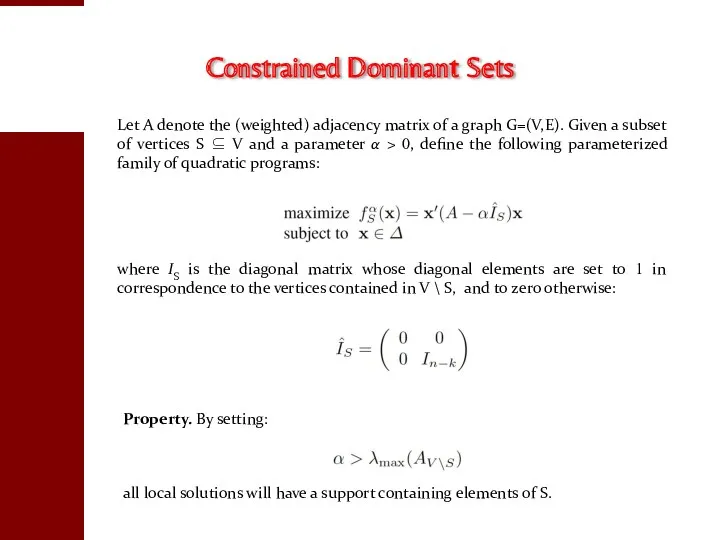
- 106. Let A denote the (weighted) adjacency matrix of a graph G=(V,E). Given a subset of vertices
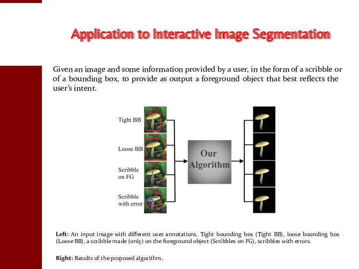
- 107. Left: An input image with different user annotations. Tight bounding box (Tight BB), loose bounding box
- 108. Left: Over-segmented image with a user scribble (blue label). Middle: The corresponding affinity matrix, using each
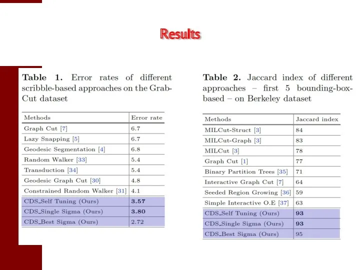
- 109. Results
- 110. Bounding box Result Scribble Result Ground truth Results
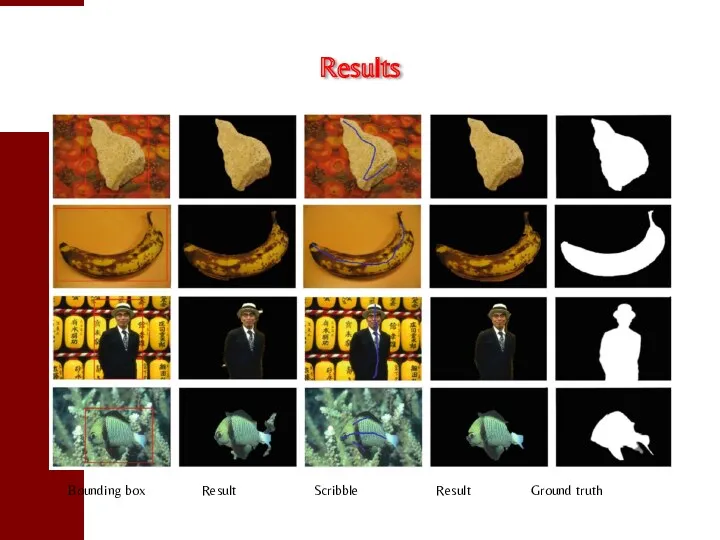
- 111. Bounding box Result Scribble Result Ground truth Results
- 112. The “protein function predition” game Motivation: network-based methods for the automatic prediction of protein functions can
- 113. Protein similarity The similarity between proteins has been calculated integrating different data types. The final similarity
- 114. Funtion similarity The similarities between the classes functionalities have been computed using the Gene Ontology (GO)
- 116. Скачать презентацию
From Cliques to Equilibria
Dominant-Set Clustering and Its Applications
From Cliques to Equilibria
Dominant-Set Clustering and Its Applications
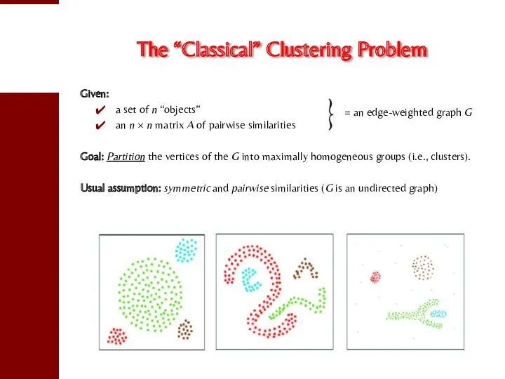
The “Classical” Clustering Problem
Given:
a set of n “objects”
an n × n
The “Classical” Clustering Problem
Given:
a set of n “objects”
an n × n
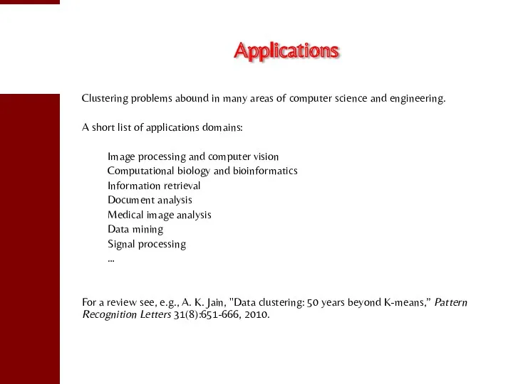
Applications
Clustering problems abound in many areas of computer science and engineering.
A
Applications
Clustering problems abound in many areas of computer science and engineering.
A
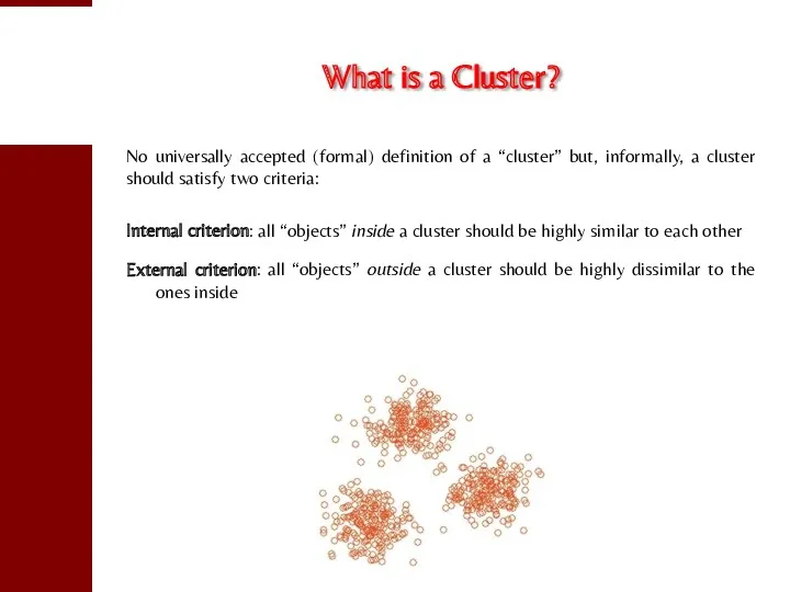
What is a Cluster?
No universally accepted (formal) definition of a “cluster”
What is a Cluster?
No universally accepted (formal) definition of a “cluster”
A Special Case:
Binary Symmetric Similarities
Suppose the similarity matrix is a binary
A Special Case:
Binary Symmetric Similarities
Suppose the similarity matrix is a binary
Advantages of the New Approach
No need to know the number of
Advantages of the New Approach
No need to know the number of
What is Game Theory?
A few cornerstones in game theory
1921−1928: Emile Borel
What is Game Theory?
A few cornerstones in game theory
1921−1928: Emile Borel
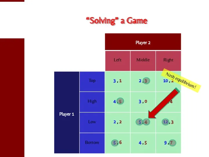
“Solving” a Game
Nash equilibrium!
“Solving” a Game
Nash equilibrium!
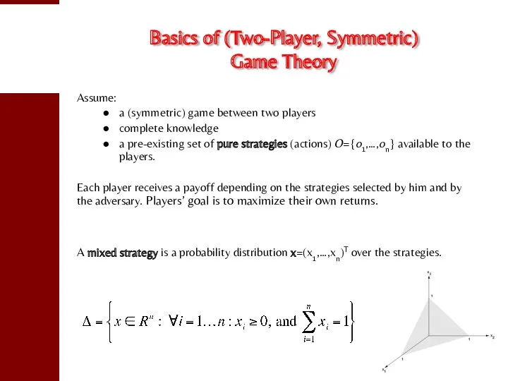
Basics of (Two-Player, Symmetric)
Game Theory
Assume:
a (symmetric) game between two players
complete
Basics of (Two-Player, Symmetric)
Game Theory
Assume:
a (symmetric) game between two players
complete
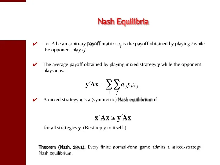
Nash Equilibria
Let A be an arbitrary payoff matrix: aij is the
Nash Equilibria
Let A be an arbitrary payoff matrix: aij is the
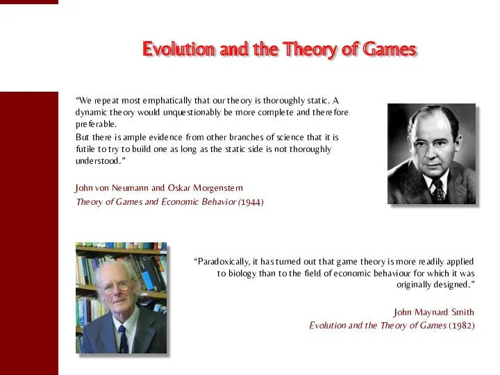
Evolution and the Theory of Games
“We repeat most emphatically that our
Evolution and the Theory of Games
“We repeat most emphatically that our
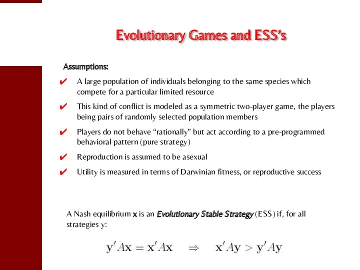
Evolutionary Games and ESS’s
Assumptions:
A large population of individuals belonging to the
Evolutionary Games and ESS’s
Assumptions:
A large population of individuals belonging to the
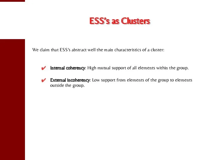
ESS’s as Clusters
We claim that ESS’s abstract well the main characteristics
ESS’s as Clusters
We claim that ESS’s abstract well the main characteristics
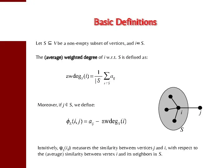
Basic Definitions
Let S ⊆ V be a non-empty subset of vertices,
Basic Definitions
Let S ⊆ V be a non-empty subset of vertices,
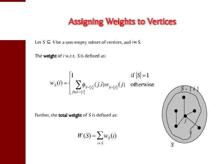
Assigning Weights to Vertices
Let S ⊆ V be a non-empty subset
Assigning Weights to Vertices
Let S ⊆ V be a non-empty subset
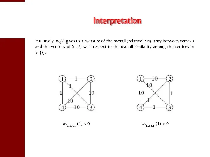
Interpretation
Intuitively, wS(i) gives us a measure of the overall (relative) similarity
Interpretation
Intuitively, wS(i) gives us a measure of the overall (relative) similarity
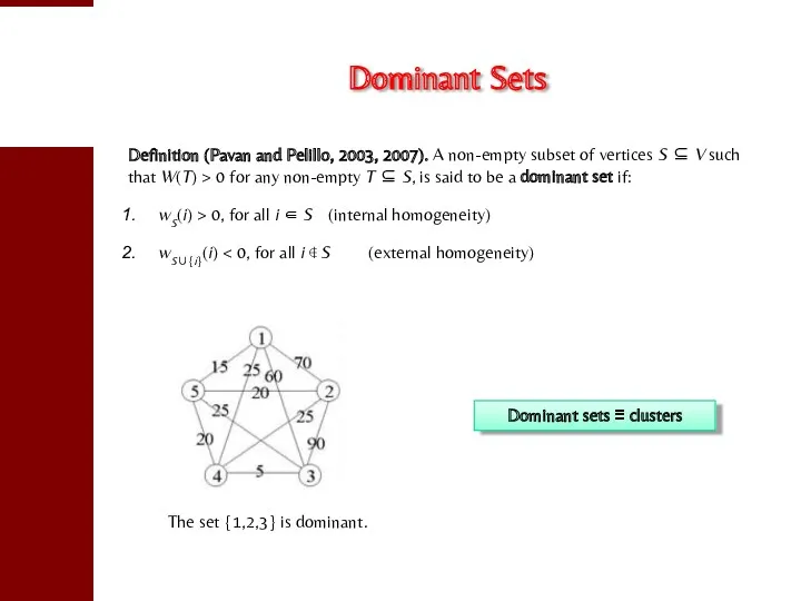
Dominant Sets
Definition (Pavan and Pelillo, 2003, 2007). A non-empty subset of
Dominant Sets
Definition (Pavan and Pelillo, 2003, 2007). A non-empty subset of
The Clustering Game
Consider the following “clustering game.”
Assume a preexisting set
The Clustering Game
Consider the following “clustering game.”
Assume a preexisting set
Dominant Sets are ESS’s
Theorem (Torsello, Rota Bulò and Pelillo, 2006). Evolutionary
Dominant Sets are ESS’s
Theorem (Torsello, Rota Bulò and Pelillo, 2006). Evolutionary
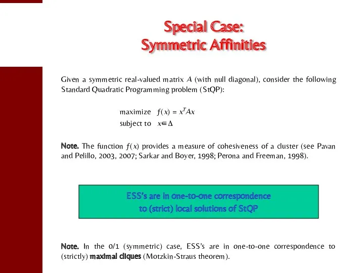
Special Case:
Symmetric Affinities
Given a symmetric real-valued matrix A (with null diagonal),
Special Case:
Symmetric Affinities
Given a symmetric real-valued matrix A (with null diagonal),
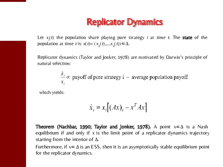
Replicator Dynamics
Let xi(t) the population share playing pure strategy i at
Replicator Dynamics
Let xi(t) the population share playing pure strategy i at
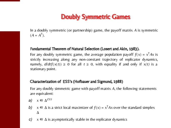
Doubly Symmetric Games
In a doubly symmetric (or partnership) game, the payoff
Doubly Symmetric Games
In a doubly symmetric (or partnership) game, the payoff
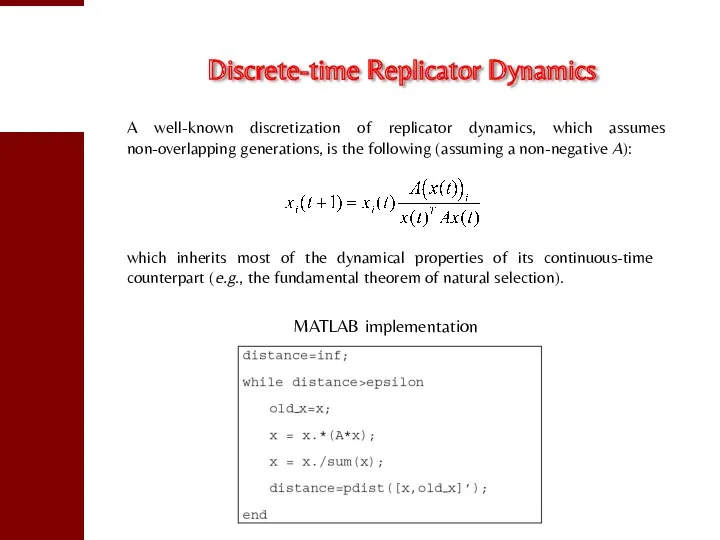
Discrete-time Replicator Dynamics
A well-known discretization of replicator dynamics, which assumes non-overlapping
Discrete-time Replicator Dynamics
A well-known discretization of replicator dynamics, which assumes non-overlapping
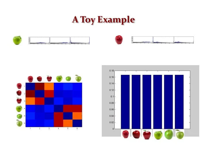
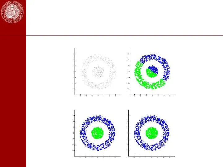
A Toy Example
A Toy Example
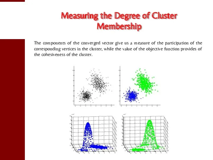
Measuring the Degree of Cluster Membership
The components of the converged vector
Measuring the Degree of Cluster Membership
The components of the converged vector
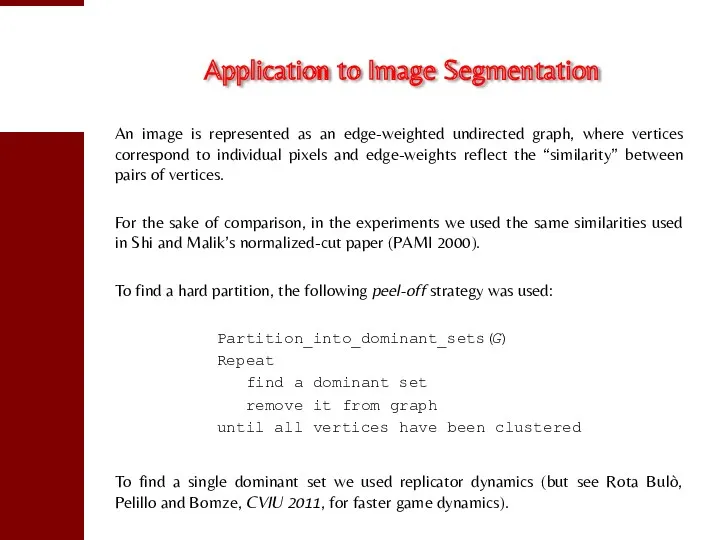
Application to Image Segmentation
An image is represented as an edge-weighted undirected
Application to Image Segmentation
An image is represented as an edge-weighted undirected
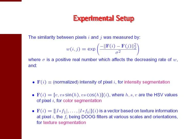
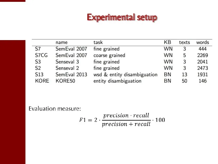
Experimental Setup
Experimental Setup
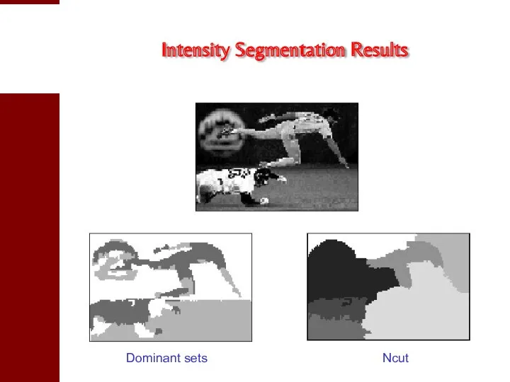
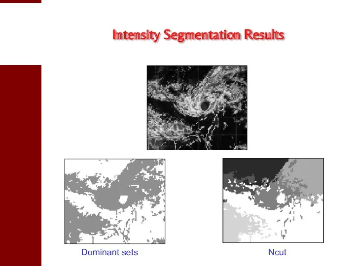
Intensity Segmentation Results
Dominant sets
Ncut
Intensity Segmentation Results
Dominant sets
Ncut
Intensity Segmentation Results
Dominant sets Ncut
Intensity Segmentation Results
Dominant sets Ncut
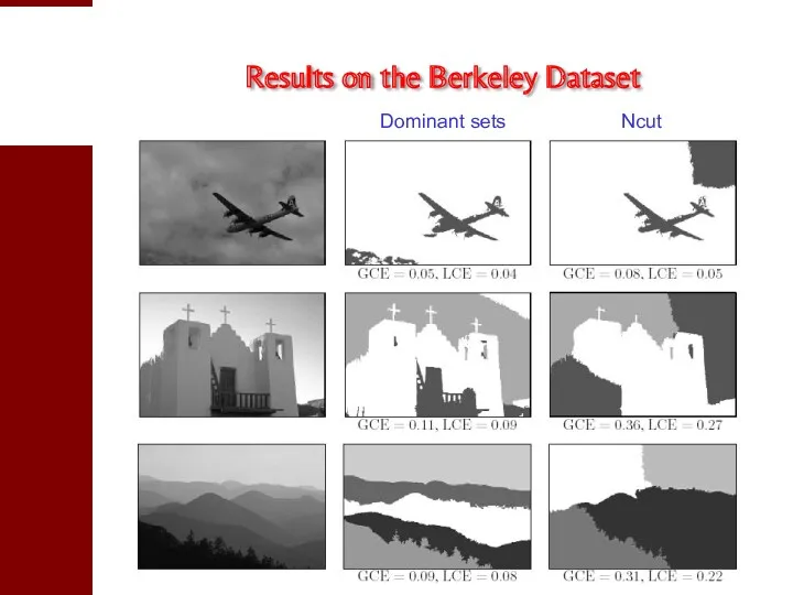
Results on the Berkeley Dataset
Dominant sets Ncut
Results on the Berkeley Dataset
Dominant sets Ncut
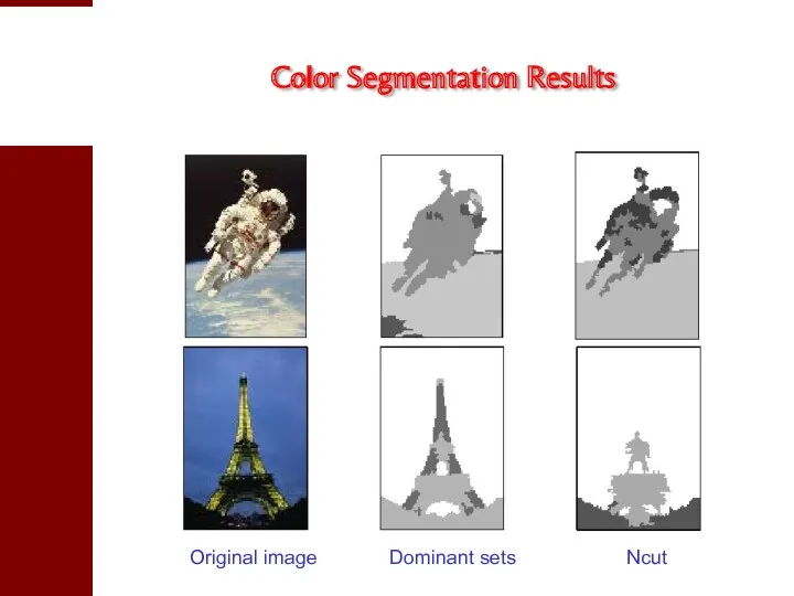
Color Segmentation Results
Original image Dominant sets Ncut
Color Segmentation Results
Original image Dominant sets Ncut
Dominant sets Ncut
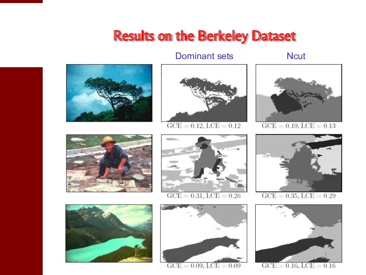
Results on the Berkeley Dataset
Dominant sets Ncut
Results on the Berkeley Dataset
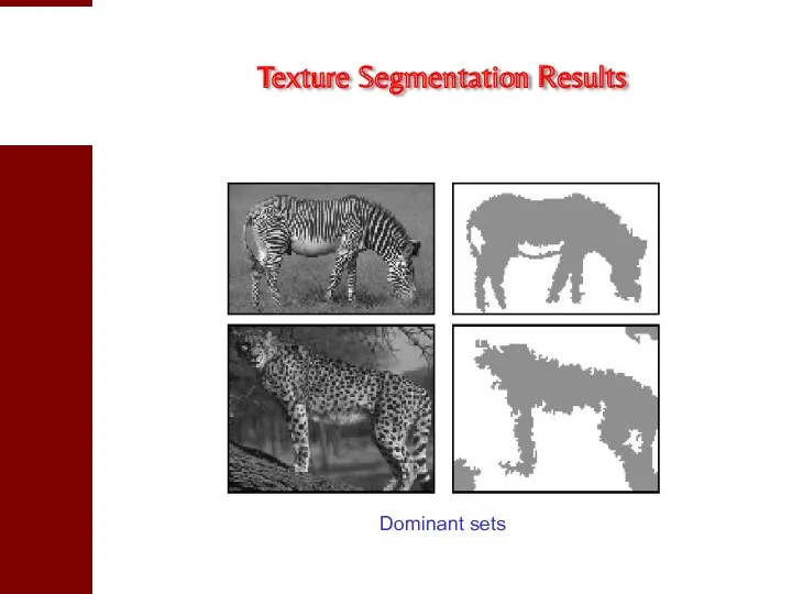
Texture Segmentation Results
Dominant sets
Texture Segmentation Results
Dominant sets
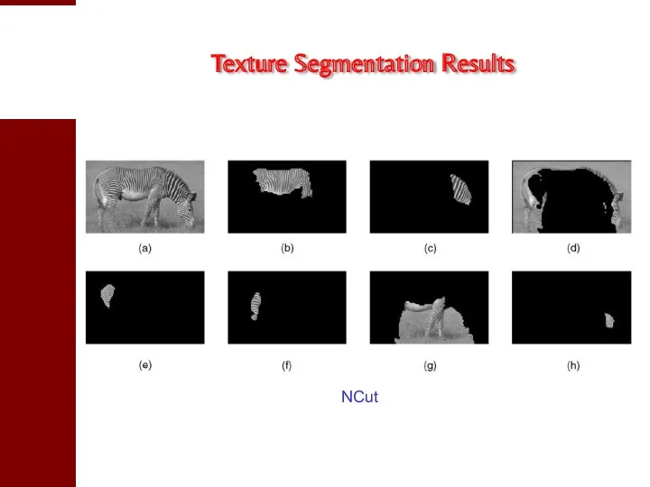
Texture Segmentation Results
NCut
Texture Segmentation Results
NCut
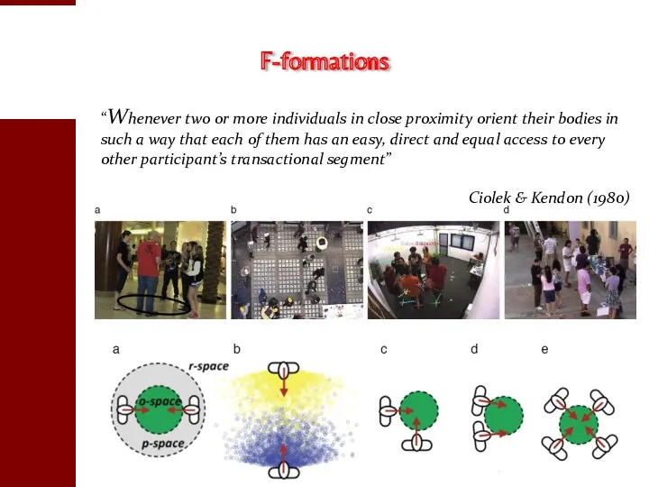
F-formations
“Whenever two or more individuals in close proximity orient their bodies
F-formations
“Whenever two or more individuals in close proximity orient their bodies
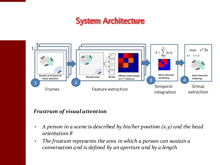
System Architecture
Frustrum of visual attention
A person in a scene is described
System Architecture
Frustrum of visual attention
A person in a scene is described
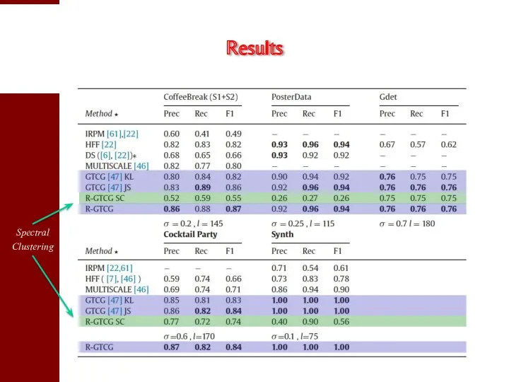
Results
Results
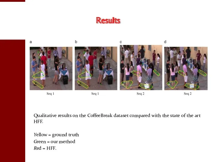
Qualitative results on the CoffeeBreak dataset compared with the state of
Qualitative results on the CoffeeBreak dataset compared with the state of
Bioinformatics
Identification of protein binding sites (Zauhar and Bruist, 2005)
Clustering gene expression
Bioinformatics
Identification of protein binding sites (Zauhar and Bruist, 2005)
Clustering gene expression

Extensions
Extensions
First idea: run replicator dynamics from different starting points in the
First idea: run replicator dynamics from different starting points in the
Finding Overlapping Classes:
Intuition
Finding Overlapping Classes:
Intuition
Building a Hierarchy:
A Family of Quadratic Programs
Building a Hierarchy:
A Family of Quadratic Programs
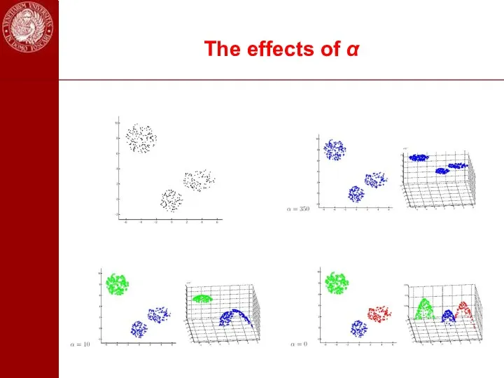
The effects of α
The effects of α
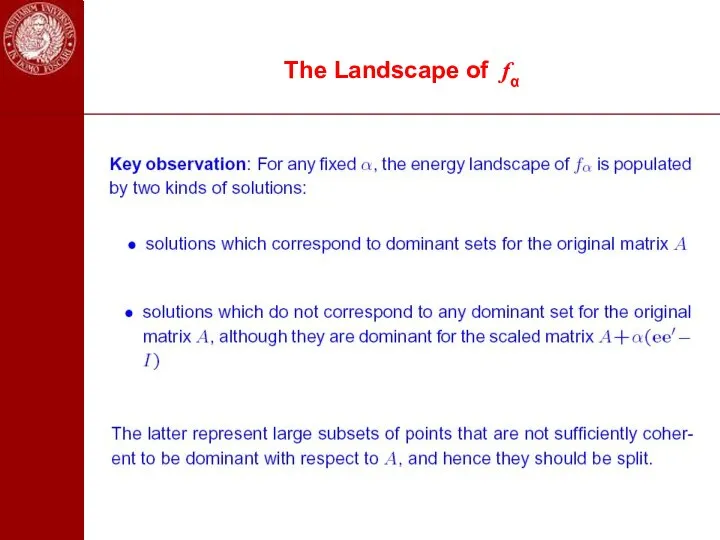
The Landscape of fα
The Landscape of fα
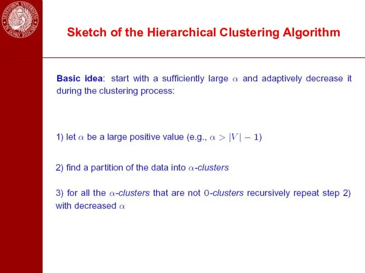
Sketch of the Hierarchical Clustering Algorithm
Sketch of the Hierarchical Clustering Algorithm
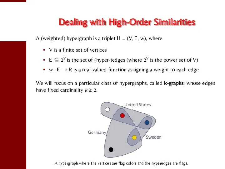
Dealing with High-Order Similarities
A (weighted) hypergraph is a triplet H
Dealing with High-Order Similarities
A (weighted) hypergraph is a triplet H
The Hypergraph Clustering Game
Given a weighted k-graph representing an instance of
The Hypergraph Clustering Game
Given a weighted k-graph representing an instance of
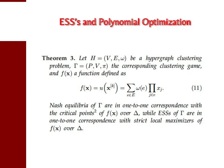
ESS’s and Polynomial Optimization
ESS’s and Polynomial Optimization
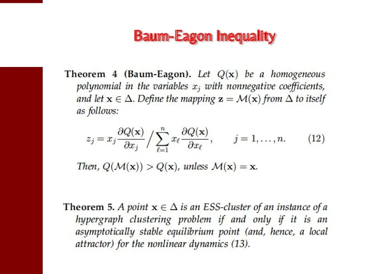
Baum-Eagon Inequality
Baum-Eagon Inequality
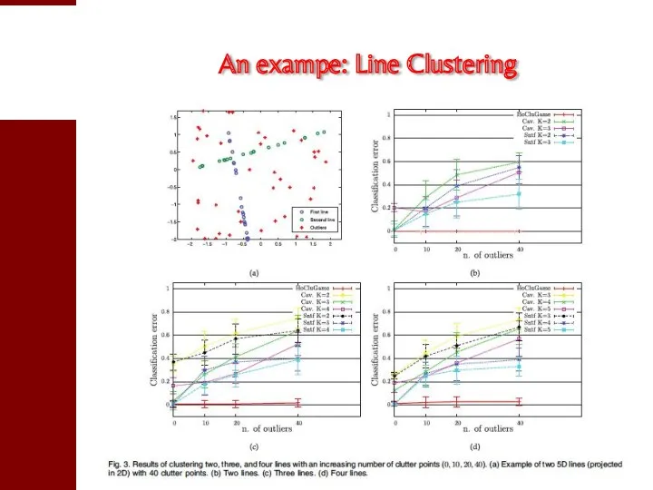
An exampe: Line Clustering
An exampe: Line Clustering
In a nutshell…
The game-theoretic/dominant-set approach:
makes no assumption on the structure of
In a nutshell…
The game-theoretic/dominant-set approach:
makes no assumption on the structure of
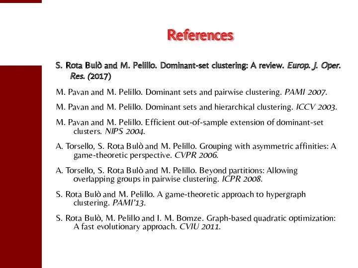
References
S. Rota Bulò and M. Pelillo. Dominant-set clustering: A review. Europ.
References
S. Rota Bulò and M. Pelillo. Dominant-set clustering: A review. Europ.
Hume-Nash Machines
Context-Aware Models of Learning and Recognition
Hume-Nash Machines
Context-Aware Models of Learning and Recognition
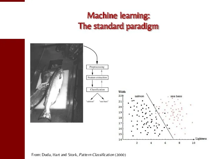
Machine learning:
The standard paradigm
From: Duda, Hart and Stork, Pattern Classification (2000)
Machine learning:
The standard paradigm
From: Duda, Hart and Stork, Pattern Classification (2000)
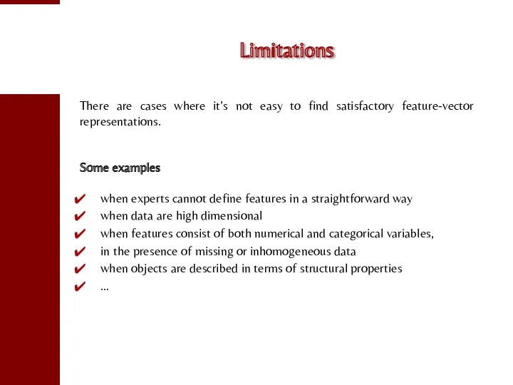
Limitations
There are cases where it’s not easy to find satisfactory feature-vector
Limitations
There are cases where it’s not easy to find satisfactory feature-vector
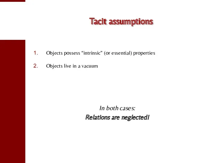
Tacit assumptions
Objects possess “intrinsic” (or essential) properties
Objects live in a vacuum
In
Tacit assumptions
Objects possess “intrinsic” (or essential) properties
Objects live in a vacuum
In
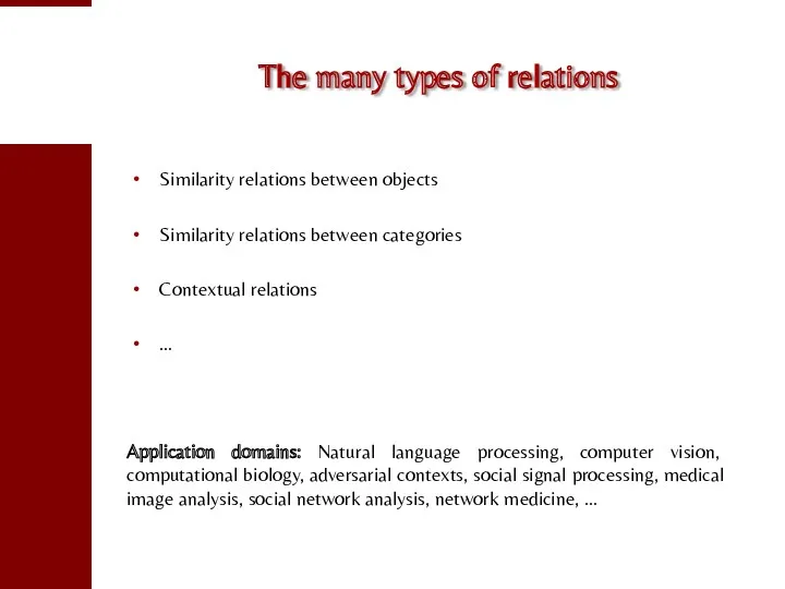
The many types of relations
Similarity relations between objects
Similarity relations between categories
Contextual
The many types of relations
Similarity relations between objects
Similarity relations between categories
Contextual
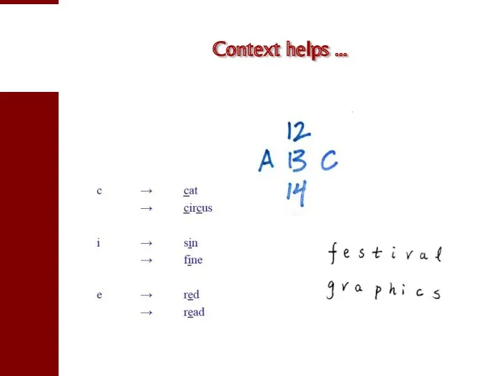
Context helps …
Context helps …
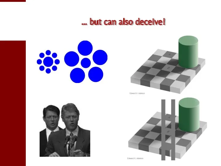
… but can also deceive!
… but can also deceive!
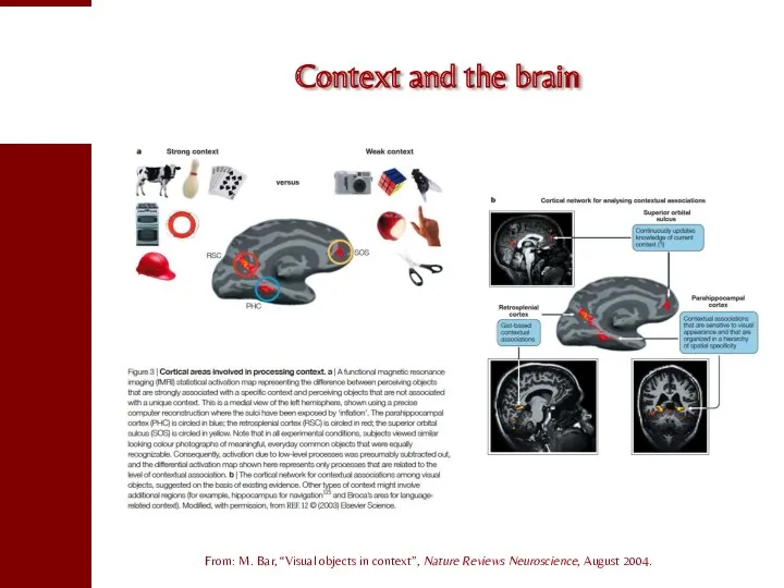
Context and the brain
From: M. Bar, “Visual objects in context”, Nature
Context and the brain
From: M. Bar, “Visual objects in context”, Nature
Beyond features?
The field is showing an increasing propensity towards relational approaches,
Beyond features?
The field is showing an increasing propensity towards relational approaches,
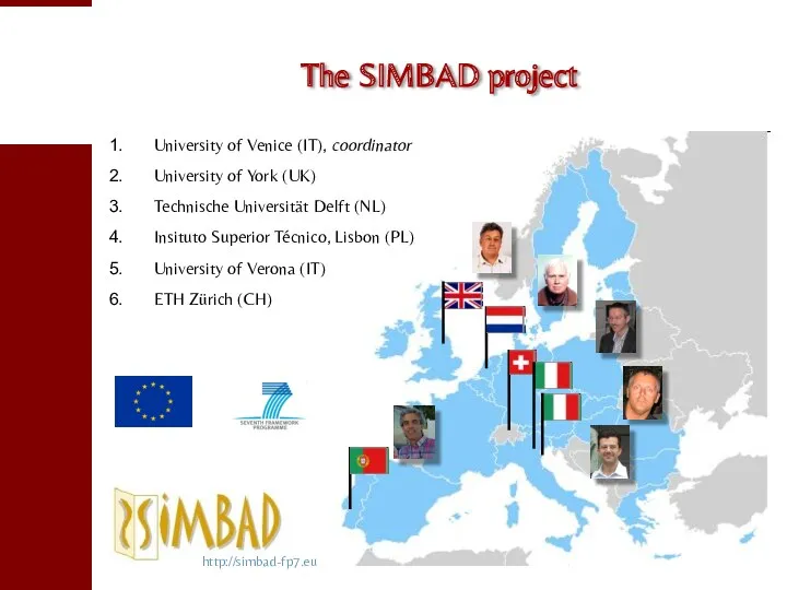
The SIMBAD project
University of Venice (IT), coordinator
University of York (UK)
Technische Universität
The SIMBAD project
University of Venice (IT), coordinator
University of York (UK)
Technische Universität
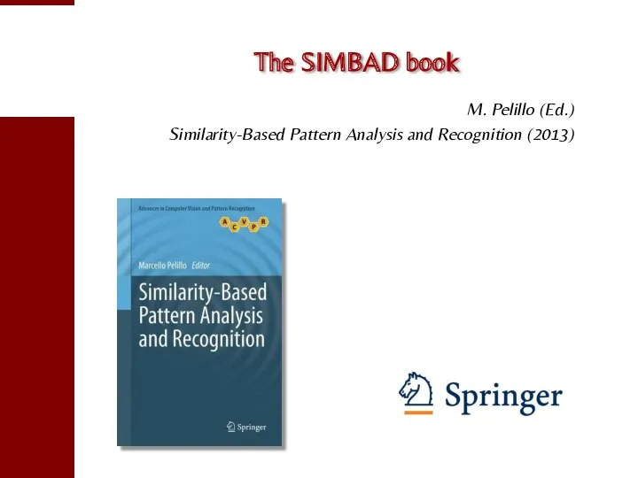
The SIMBAD book
M. Pelillo (Ed.)
Similarity-Based Pattern Analysis and Recognition (2013)
The SIMBAD book
M. Pelillo (Ed.)
Similarity-Based Pattern Analysis and Recognition (2013)
Challenges to similarity-based approaches
Departing from vector-space representations:
dealing with (dis)similarities that might
Challenges to similarity-based approaches
Departing from vector-space representations:
dealing with (dis)similarities that might
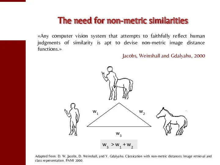
The need for non-metric similarities
«Any computer vision system that attempts to
The need for non-metric similarities
«Any computer vision system that attempts to
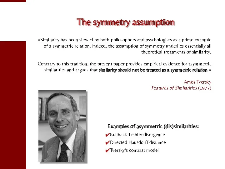
The symmetry assumption
«Similarity has been viewed by both philosophers and psychologists
The symmetry assumption
«Similarity has been viewed by both philosophers and psychologists
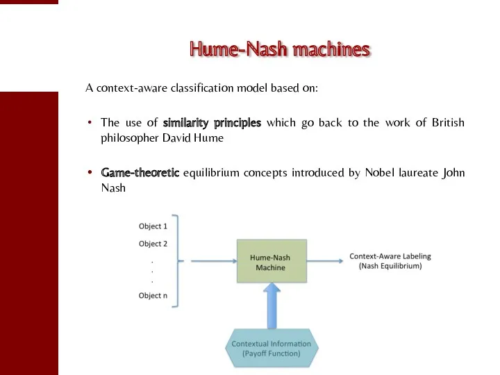
Hume-Nash machines
A context-aware classification model based on:
The use of similarity principles
Hume-Nash machines
A context-aware classification model based on:
The use of similarity principles
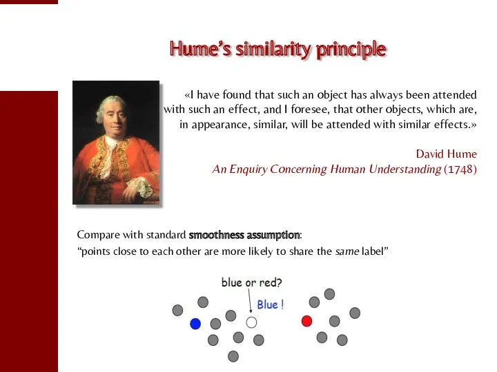
Hume’s similarity principle
«I have found that such an object has always
Hume’s similarity principle
«I have found that such an object has always
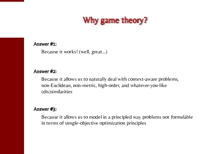
Why game theory?
Answer #1:
Because it works! (well, great…)
Answer #3:
Because it allows
Why game theory?
Answer #1:
Because it works! (well, great…)
Answer #3:
Because it allows
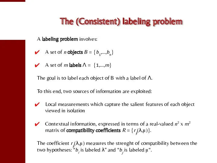
The (Consistent) labeling problem
A labeling problem involves:
A set of n objects
The (Consistent) labeling problem
A labeling problem involves:
A set of n objects
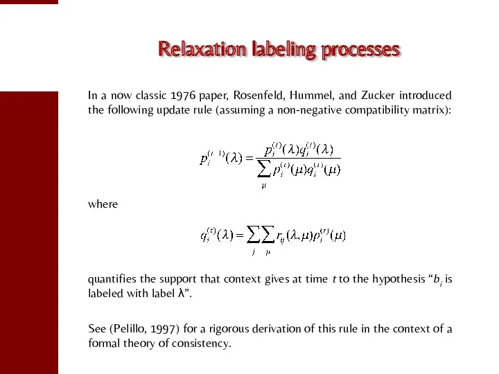
Relaxation labeling processes
In a now classic 1976 paper, Rosenfeld, Hummel, and
Relaxation labeling processes
In a now classic 1976 paper, Rosenfeld, Hummel, and
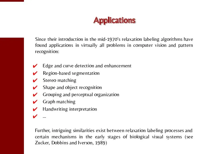
Applications
Since their introduction in the mid-1970’s relaxation labeling algorithms have found
Applications
Since their introduction in the mid-1970’s relaxation labeling algorithms have found
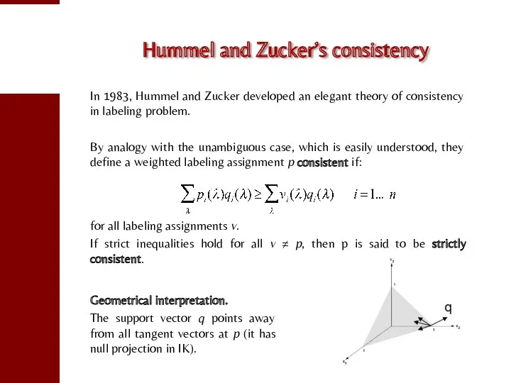
Hummel and Zucker’s consistency
In 1983, Hummel and Zucker developed an elegant
Hummel and Zucker’s consistency
In 1983, Hummel and Zucker developed an elegant
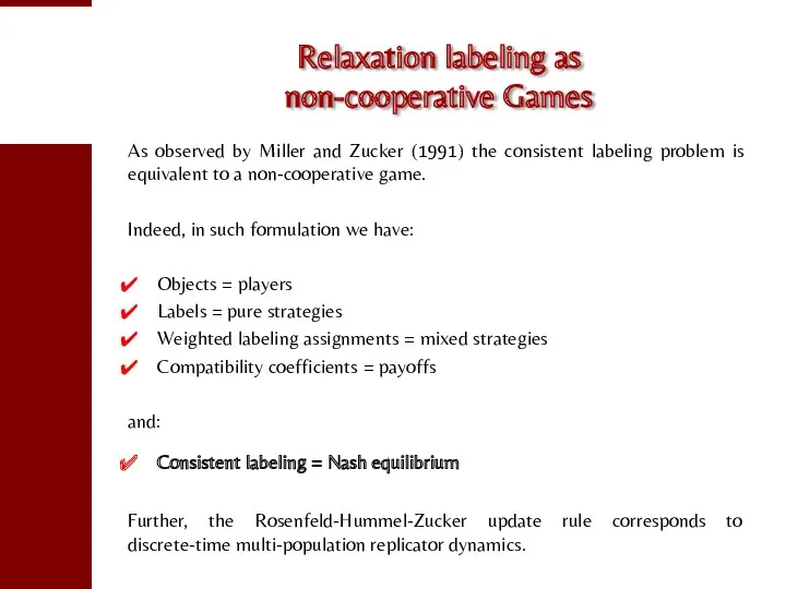
Relaxation labeling as
non-cooperative Games
As observed by Miller and Zucker (1991) the
Relaxation labeling as
non-cooperative Games
As observed by Miller and Zucker (1991) the
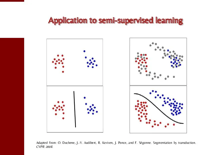
Application to semi-supervised learning
Adapted from: O. Duchene, J.-Y. Audibert, R. Keriven,
Application to semi-supervised learning
Adapted from: O. Duchene, J.-Y. Audibert, R. Keriven,
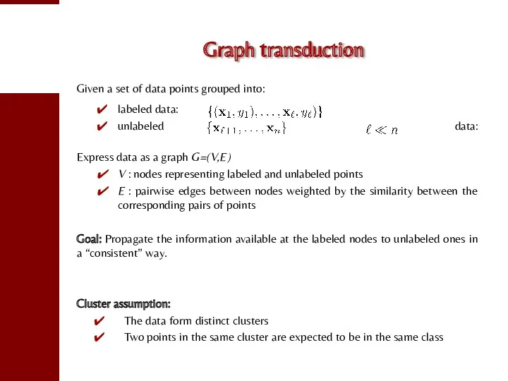
Graph transduction
Given a set of data points grouped into:
labeled data:
Graph transduction
Given a set of data points grouped into:
labeled data:
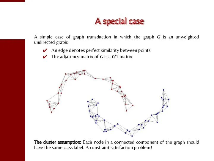
A special case
A simple case of graph transduction in which the
A special case
A simple case of graph transduction in which the
The graph transduction game
Given a weighted graph G = (V, E,
The graph transduction game
Given a weighted graph G = (V, E,
In short…
Graph transduction can be formulated as a non-cooperative game (i.e.,
In short…
Graph transduction can be formulated as a non-cooperative game (i.e.,
Extensions
The approach described here is being naturally extended along several directions:
Using
Extensions
The approach described here is being naturally extended along several directions:
Using
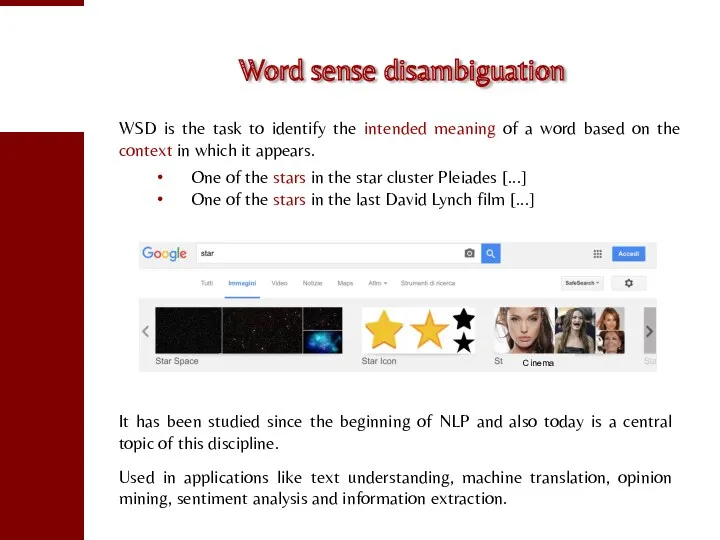
Word sense disambiguation
WSD is the task to identify the intended meaning
Word sense disambiguation
WSD is the task to identify the intended meaning
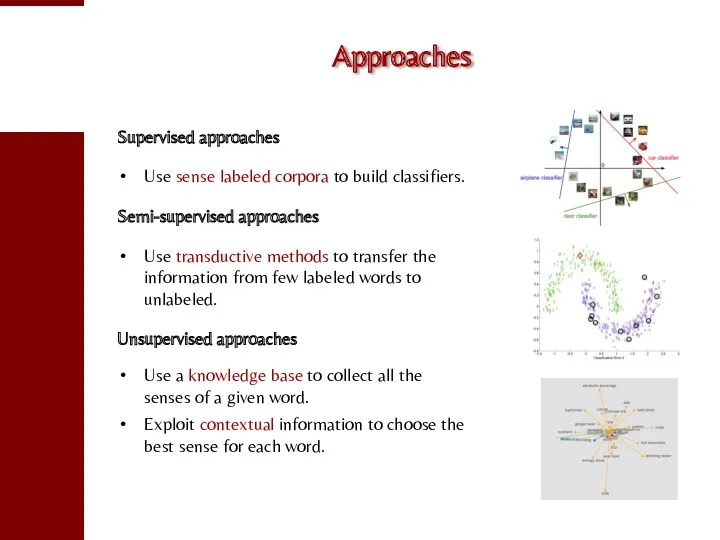
Approaches
Supervised approaches
Use sense labeled corpora to build classifiers.
Semi-supervised approaches
Use transductive methods
Approaches
Supervised approaches
Use sense labeled corpora to build classifiers.
Semi-supervised approaches
Use transductive methods
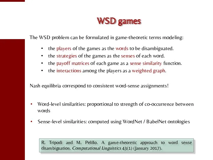
WSD games
The WSD problem can be formulated in game-theoretic terms modeling:
WSD games
The WSD problem can be formulated in game-theoretic terms modeling:
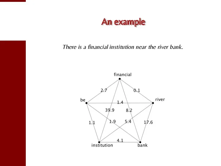
An example
There is a financial institution near the river bank.
An example
There is a financial institution near the river bank.
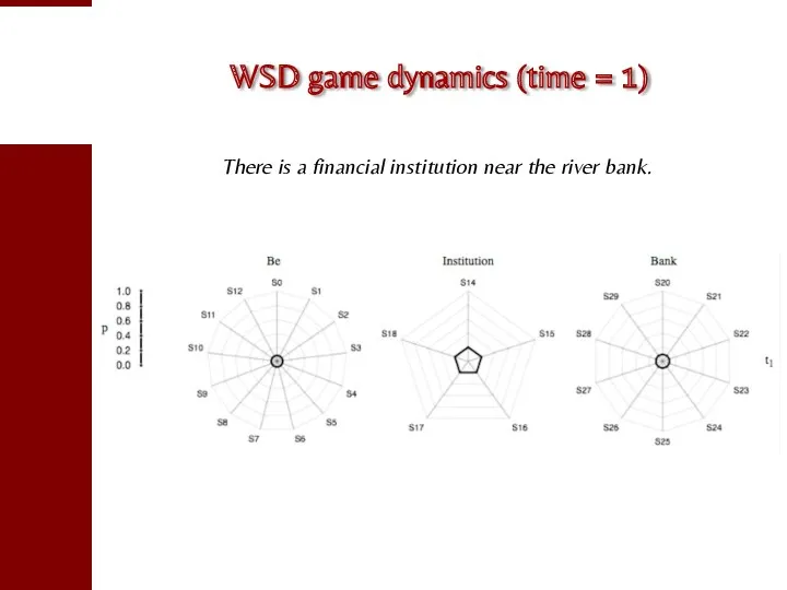
WSD game dynamics (time = 1)
There is a financial institution near
WSD game dynamics (time = 1)
There is a financial institution near
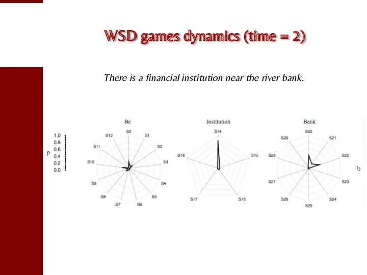
WSD games dynamics (time = 2)
There is a financial institution near
WSD games dynamics (time = 2)
There is a financial institution near

WSD game dynamics (time = 3)
There is a financial institution near
WSD game dynamics (time = 3)
There is a financial institution near
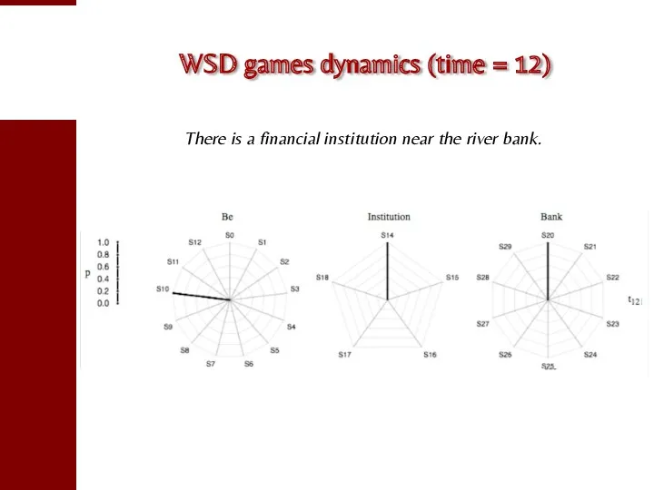
WSD games dynamics (time = 12)
There is a financial institution near
WSD games dynamics (time = 12)
There is a financial institution near
Experimental setup
Experimental setup
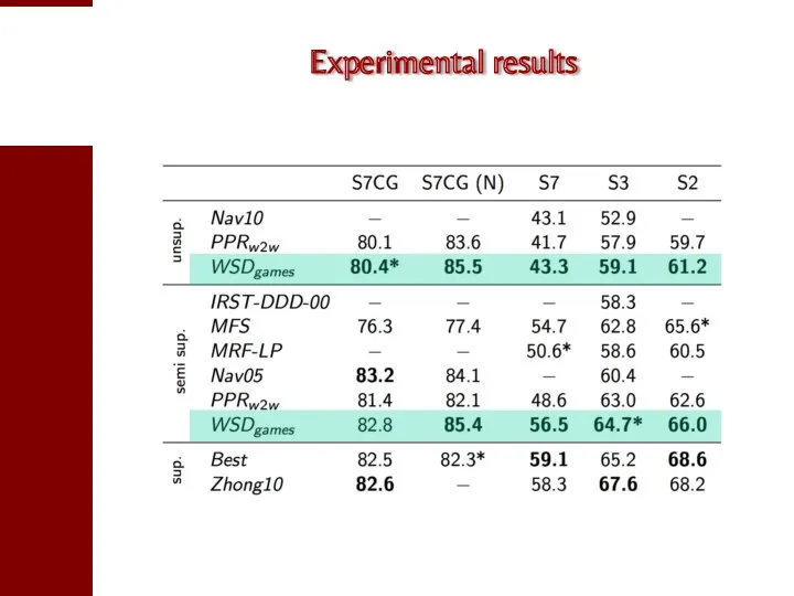
Experimental results
Experimental results
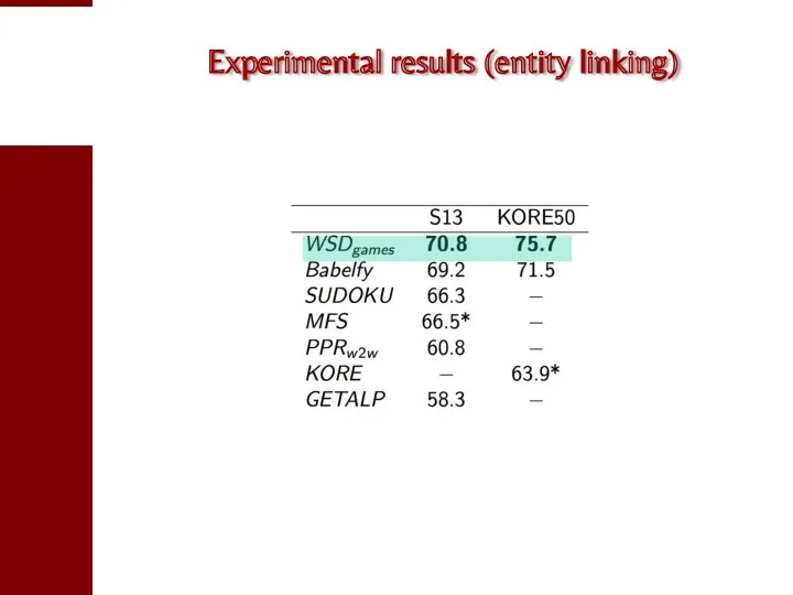
Experimental results (entity linking)
Experimental results (entity linking)
To sum up
Game theory offers a principled and viable solution to
To sum up
Game theory offers a principled and viable solution to
References
A. Rosenfeld, R. A. Hummel, and S. W. Zucker. Scene labeling
References
A. Rosenfeld, R. A. Hummel, and S. W. Zucker. Scene labeling
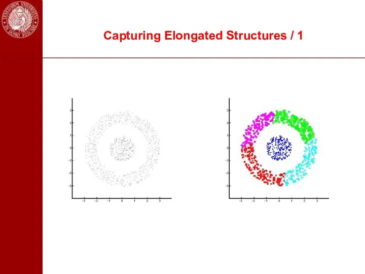
Capturing Elongated Structures / 1
Capturing Elongated Structures / 1
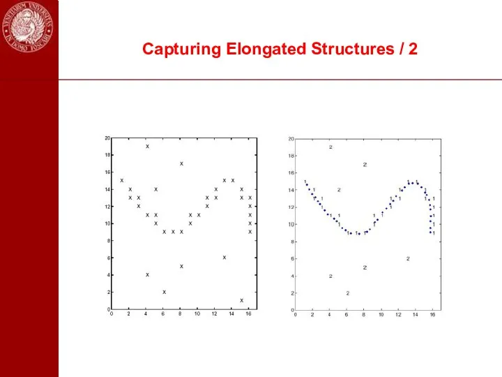
Capturing Elongated Structures / 2
Capturing Elongated Structures / 2
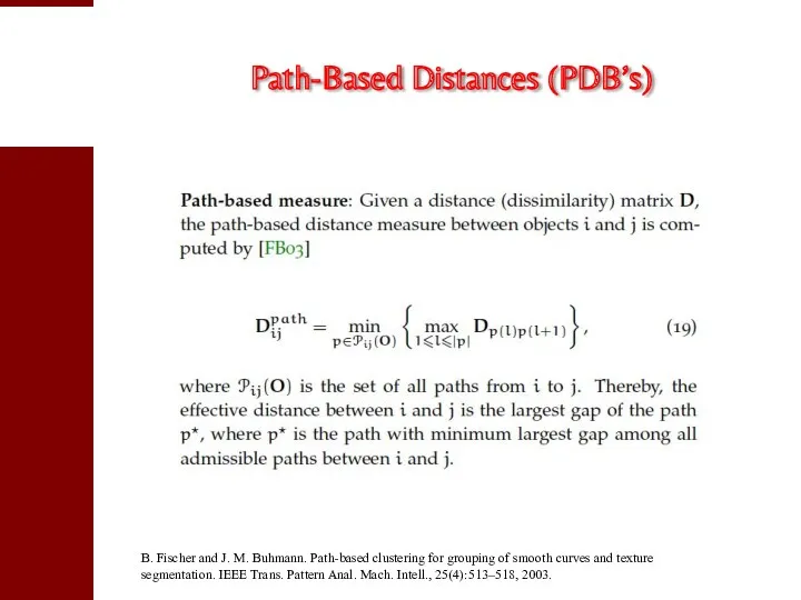
Path-Based Distances (PDB’s)
B. Fischer and J. M. Buhmann. Path-based clustering
Path-Based Distances (PDB’s)
B. Fischer and J. M. Buhmann. Path-based clustering
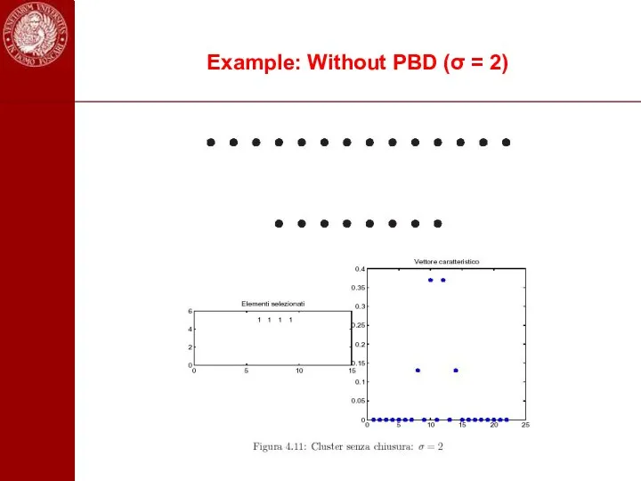
Example: Without PBD (σ = 2)
Example: Without PBD (σ = 2)
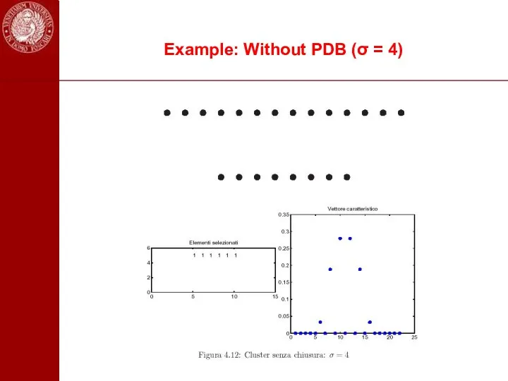
Example: Without PDB (σ = 4)
Example: Without PDB (σ = 4)
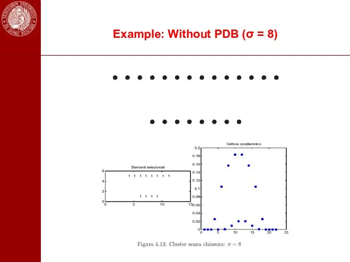
Example: Without PDB (σ = 8)
Example: Without PDB (σ = 8)
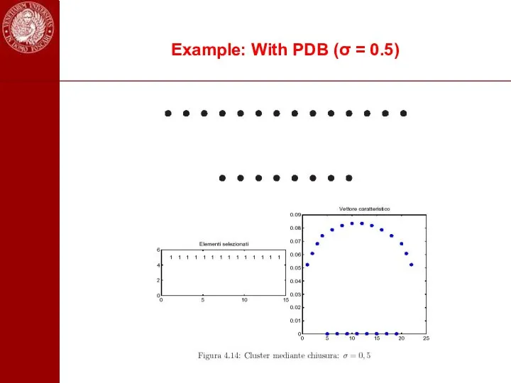
Example: With PDB (σ = 0.5)
Example: With PDB (σ = 0.5)
Let A denote the (weighted) adjacency matrix of a graph G=(V,E).
Let A denote the (weighted) adjacency matrix of a graph G=(V,E).
Left: An input image with different user annotations. Tight bounding box
Left: An input image with different user annotations. Tight bounding box
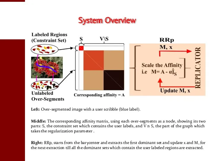
Left: Over-segmented image with a user scribble (blue label).
Middle: The
Left: Over-segmented image with a user scribble (blue label).
Middle: The
Results
Results
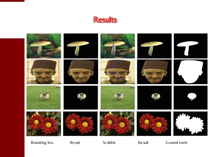
Bounding box Result Scribble Result Ground truth
Results
Bounding box Result Scribble Result Ground truth
Results
Bounding box Result Scribble Result Ground truth
Results
Bounding box Result Scribble Result Ground truth
Results

The “protein function predition” game
Motivation: network-based methods for the automatic prediction
The “protein function predition” game
Motivation: network-based methods for the automatic prediction
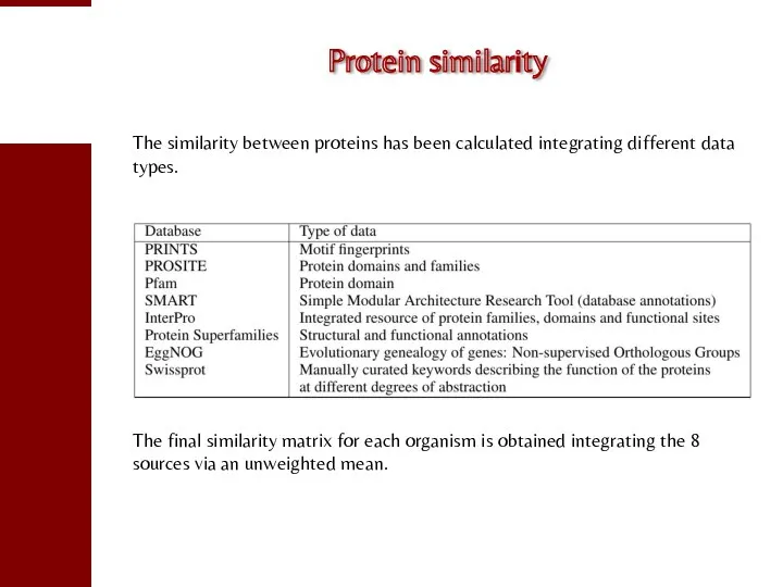
Protein similarity
The similarity between proteins has been calculated integrating different data
Protein similarity
The similarity between proteins has been calculated integrating different data
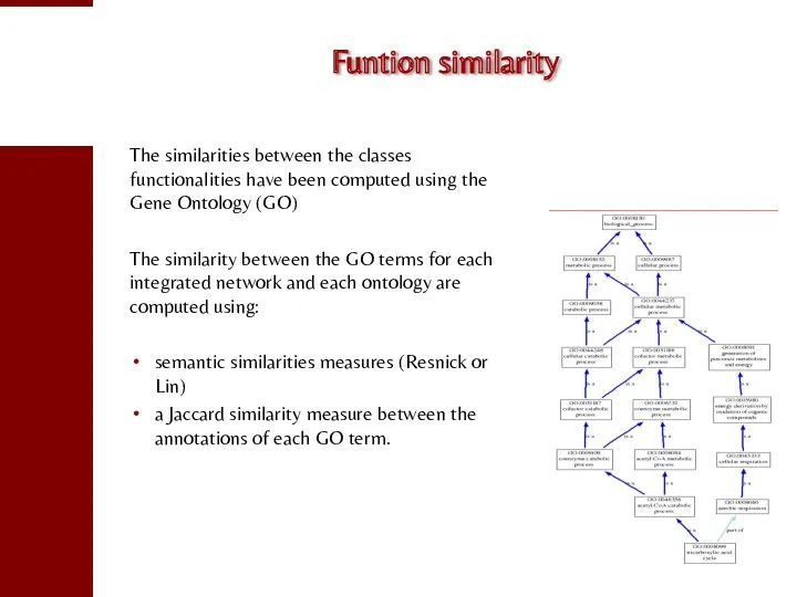
Funtion similarity
The similarities between the classes functionalities have been computed using
Funtion similarity
The similarities between the classes functionalities have been computed using
 Базы данных и SQL. Семинар 3
 Инструкция по запуску дистанционных курсов
 Электронная почта и другие сервисы компьютерных сетей
 Геоинформационные системы для будущего Тольятти: взгляд горожанина
 Запуск рекламы в Instagram
 Основы программирования на С#. (Лекция 5)
 Открытый урок по информатике Алгоритм ветвления 9 класс
 Технологии искусственного интеллекта: машинное обучение. Лекция 7
 Z-преобразование
 Модель OSI. Инфокоммуникационные системы и сети
 Презентация.Логические законы.
 Автоматизированные системы управления в гостиничных предприятиях
 Agile, Scrum подходы в управлении проектами
 Методы и технологии поиска информации в научной и образовательной деятельности
 Редактор презентаций Power Point. (Часть 1)
 Технологии 3Dпечати, применяемые на АО НПК Уралвагонзавод
 Курсы тестировщиков
 Алгоритмы
 Комп'ютерні віруси та антивірусні програмні засоби
 Базы данных в информационных системах, хранилища данных
 Формальная теория защиты информации
 Первое знакомство с компьютером
 Цифровизация и ее влияние на российскую экономику
 Динамическая маршрутизация. Протокол OSPF
 Методы построения калибровочных моделей для прогнозирования свойств индивидуальных углеводородов
 Техническое задание для создания сайта. Описание структуры
 Интеллектуальная система автоведения грузового поезда с распределенной тягой ИСАВП-РТ. Клавиатура и меню
 Основы информационной безопасности критических технологий