- Interconnect delay. (Chapter 7)

Содержание
- 2. Chapter 7 Interconnect Delay 7.1 Elmore Delay 7.2 High-order model and moment matching 7.3 Stage delay
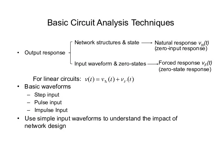
- 3. Basic Circuit Analysis Techniques Output response Basic waveforms Step input Pulse input Impulse Input Use simple
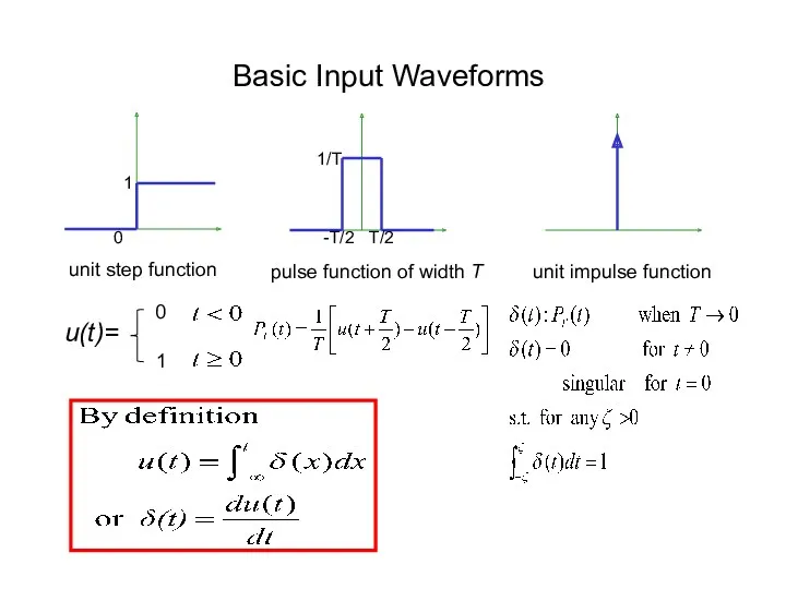
- 4. unit step function u(t)= 0 1 1 pulse function of width T 0 1/T -T/2 T/2
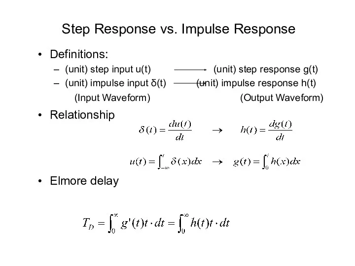
- 5. Definitions: (unit) step input u(t) (unit) step response g(t) (unit) impulse input δ(t) (unit) impulse response
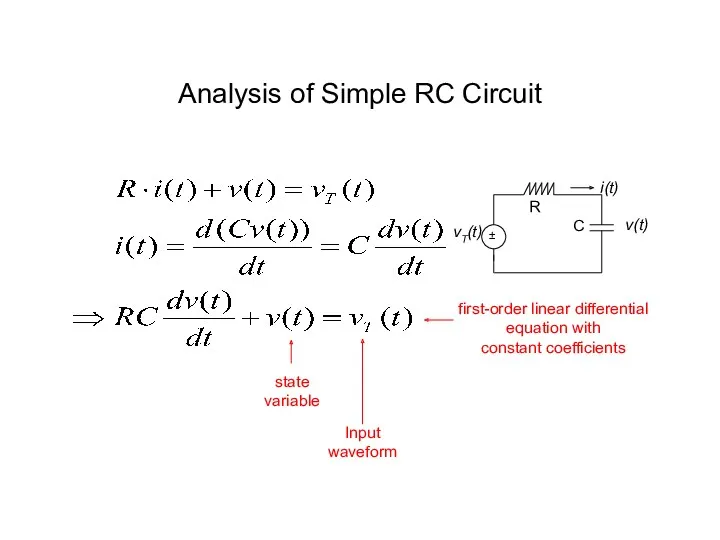
- 6. Analysis of Simple RC Circuit first-order linear differential equation with constant coefficients state variable Input waveform
- 7. Analysis of Simple RC Circuit zero-input response: (natural response) step-input response: match initial state: output response
- 8. Delays of Simple RC Circuit v(t) = v0(1 - e-t/RC) under step input v0u(t) v(t)=0.9v0 ⇒
- 9. Lumped Capacitance Delay Model R = driver resistance C = total interconnect capacitance + loading capacitance
- 10. driver Lumped RC Delay Model Minimize delay ⇔ minimize wire length Rd Cload
- 11. Delay of Distributed RC Lines Vout(t) Vout(s) Laplace Transform R VIN VOUT C VOUT VIN R
- 12. Delay of Distributed RC Lines (cont’d)
- 13. Distributed Interconnect Models Distributed RC circuit model L,T or Π circuits Distributed RCL circuit model Tree
- 14. Distributed RC Circuit Models
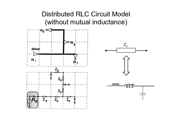
- 15. Distributed RLC Circuit Model (without mutual inductance)
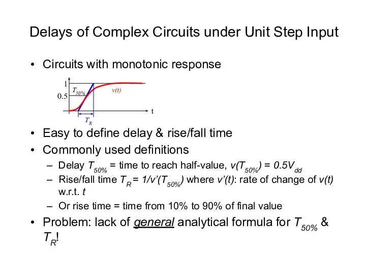
- 16. Delays of Complex Circuits under Unit Step Input Circuits with monotonic response Easy to define delay
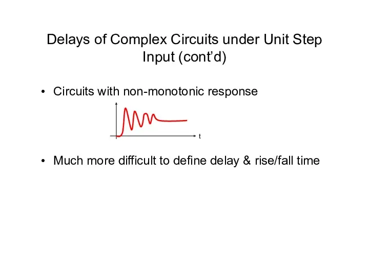
- 17. Delays of Complex Circuits under Unit Step Input (cont’d) Circuits with non-monotonic response Much more difficult
- 18. 0.5 1 T50% v(t) t t v’(t) median of v’(t) (T50%) Elmore Delay for Monotonic Responses
- 19. T50%: median of v’(t), since Elmore delay TD = mean of v’(t) Elmore Delay for Monotonic
- 20. Why Elmore Delay? Elmore delay is easier to compute analytically in most cases Elmore’s insight [Elmore,
- 21. Elmore Delay for RC Trees Definition h(t) = impulse response TD = mean of h(t) =
- 22. Elmore Delay of a RC Tree [Rubinstein-Penfield-Horowitz, T-CAD’83] Lemma: Proof: Apply impulse func. at t=0: imin
- 23. Elmore Delay in a RC Tree (cont’d) input i k j Si path resistance Rii Rjk
- 24. Elmore Delay in a RC Tree (cont’d) We shall show later on that i.e. 1-vi(T) goes
- 25. Some Definitions For Signal Bound Computation
- 26. Signal Bounds in RC Trees Theorem
- 27. Delay Bounds in RC Trees
- 28. Computation of Elmore Delay & Delay Bounds in RC Trees Let C(Tk) be total capacitance of
- 29. Comments on Elmore Delay Model Advantages Simple closed-form expression Useful for interconnect optimization Upper bound of
- 30. Comments on Elmore Delay Model Disadvantages Low accuracy, especially poor for slope computation Inherently cannot handle
- 31. Chapter 7.2 Higher-order Delay Model
- 32. Time Moments of Impulse Response h(t) Definition of moments i-th moment Note that m1 = Elmore
- 33. Pade Approximation H(s) can be modeled by Pade approximation of type (p/q): where q Or modeled
- 34. General Moment Matching Technique Basic idea: match the moments m-(2q-r), …, m-1, m0, m1, …, mr-1
- 35. Compute Residues & Poles match first 2q-1 moments EQ1
- 36. Basic Steps for Moment Matching Step 1: Compute 2q moments m-1, m0, m1, …, m(2q-2) of
- 37. Components of Moment Matching Model Moment computation Iterative DC analysis on transformed equivalent DC circuit Recursive
- 38. Chapter 7 Interconnect Delay 7.1 Elmore Delay 7.2 High-order model and moment matching 7.3 Stage delay
- 39. Stage Delay A B C Source Interconnect Load
- 40. Modeling of Capacitive Load First-order approximation: the driver sees the total capacitance of wires and sinks
- 41. Π-Model [O’Brian-Savarino, ICCAD’89] Moment matching again! Consider the first three moments of driving point admittance (moments
- 42. Driving-Point Admittance Approximations Driving-point admittance = Sum of voltage moment-weighted subtree capacitance Approximation of the driving
- 43. Driving-Point Admittance Approximations First order approximation: y(1) = sum of subtree capacitance Second order approximation: yk(2)
- 44. Third Order Approximation: Π Model
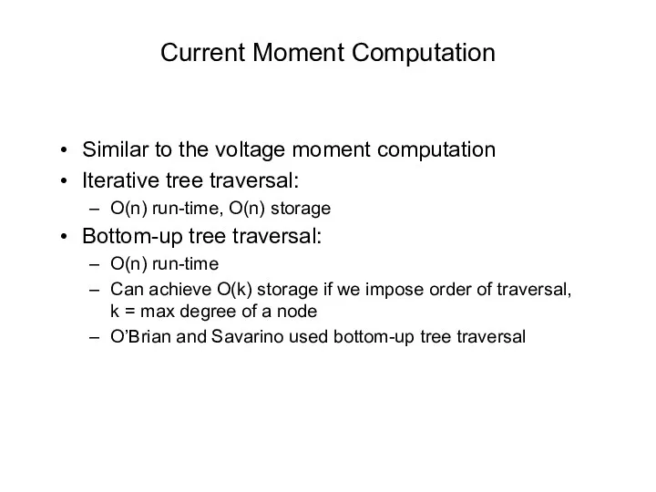
- 45. Current Moment Computation Similar to the voltage moment computation Iterative tree traversal: O(n) run-time, O(n) storage
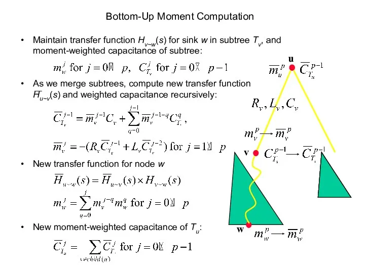
- 46. Bottom-Up Moment Computation Maintain transfer function Hv~w(s) for sink w in subtree Tv, and moment-weighted capacitance
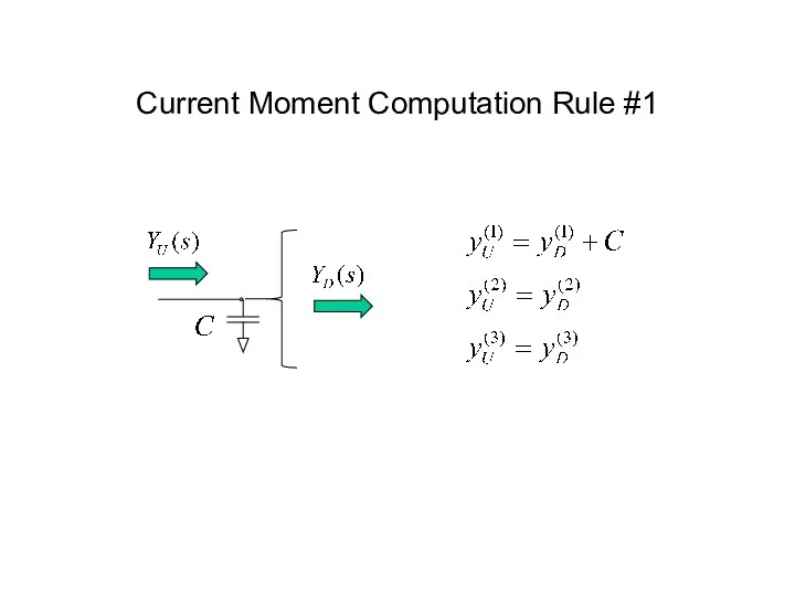
- 47. Current Moment Computation Rule #1
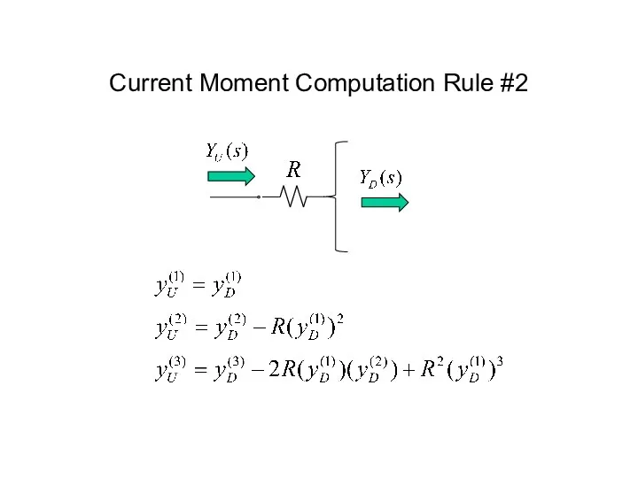
- 48. Current Moment Computation Rule #2
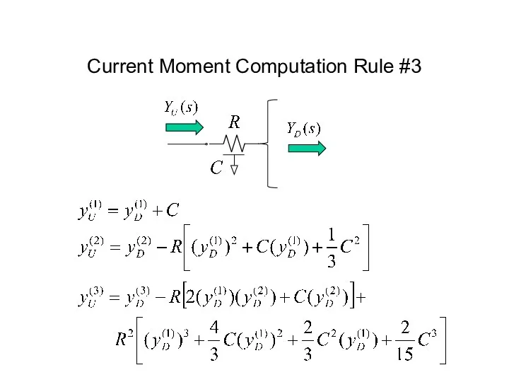
- 49. Current Moment Computation Rule #3
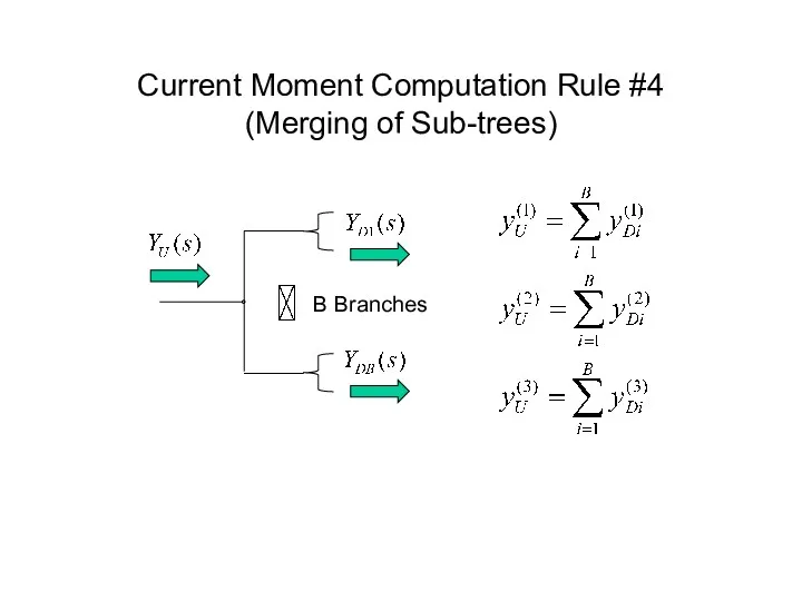
- 50. Current Moment Computation Rule #4 (Merging of Sub-trees) B Branches
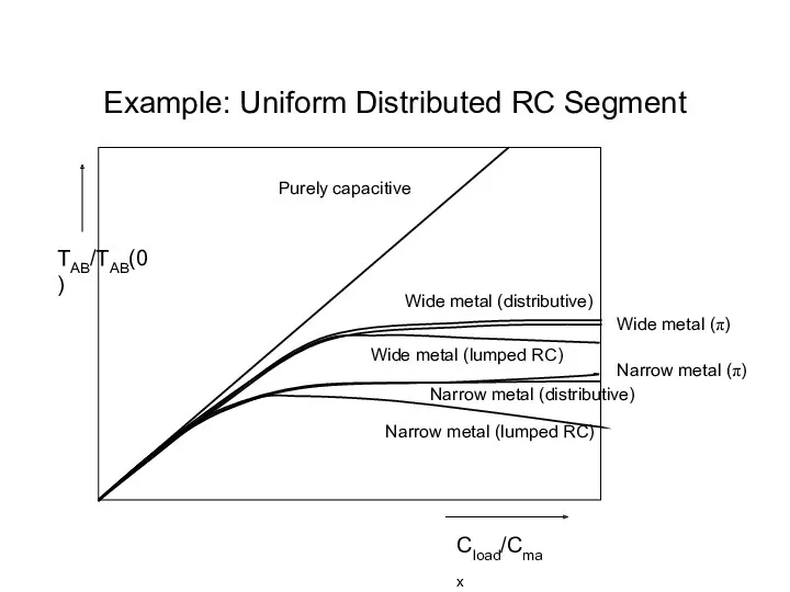
- 51. Example: Uniform Distributed RC Segment Purely capacitive Wide metal (distributive) Narrow metal (distributive) Narrow metal (lumped
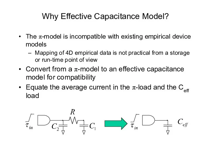
- 52. Why Effective Capacitance Model? The π-model is incompatible with existing empirical device models Mapping of 4D
- 53. Equating Average Currents tD = time taken to reach 50% point, not 50% point of input
- 54. Waveform Approximation for Vout(t) Quadratic from initial voltage (Vi = VDD for falling waveform) to 20%
- 55. Average Currents in Capacitors Average current of C1 is not quite as simple: Current due to
- 56. Average current for (0,tx) in C2 Average current for (tx,tD) in C2 Average current for (0,tD)
- 57. Computation of Effective Capacitance Equating average currents Problem: tD and tx are not known a priori
- 59. Скачать презентацию
Chapter 7 Interconnect Delay
7.1 Elmore Delay
7.2 High-order model and moment matching
7.3 Stage delay
Chapter 7 Interconnect Delay
7.1 Elmore Delay
7.2 High-order model and moment matching
7.3 Stage delay

Basic Circuit Analysis Techniques
Output response
Basic waveforms
Step input
Pulse input
Impulse Input
Use simple input waveforms to
Basic Circuit Analysis Techniques
Output response
Basic waveforms
Step input
Pulse input
Impulse Input
Use simple input waveforms to
unit step function
u(t)=
0
1
1
pulse function of width T
0
1/T
-T/2
T/2
unit impulse function
Basic Input Waveforms
unit step function
u(t)=
0
1
1
pulse function of width T
0
1/T
-T/2
T/2
unit impulse function
Basic Input Waveforms
Definitions:
(unit) step input u(t) (unit) step response g(t)
(unit) impulse input δ(t) (unit) impulse response
Definitions:
(unit) step input u(t) (unit) step response g(t)
(unit) impulse input δ(t) (unit) impulse response
Analysis of Simple RC Circuit
first-order linear differential
equation with
constant coefficients
state variable
Input
waveform
Analysis of Simple RC Circuit
first-order linear differential
equation with
constant coefficients
state variable
Input
waveform
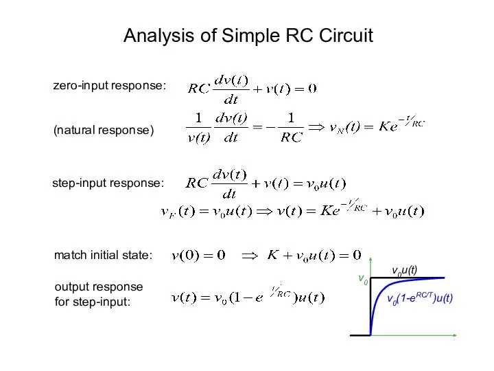
Analysis of Simple RC Circuit
zero-input response:
(natural response)
step-input response:
match initial state:
output response
for step-input:
Analysis of Simple RC Circuit
zero-input response:
(natural response)
step-input response:
match initial state:
output response
for step-input:
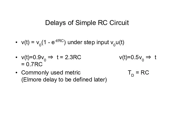
Delays of Simple RC Circuit
v(t) = v0(1 - e-t/RC) under step input v0u(t)
v(t)=0.9v0
Delays of Simple RC Circuit
v(t) = v0(1 - e-t/RC) under step input v0u(t)
v(t)=0.9v0
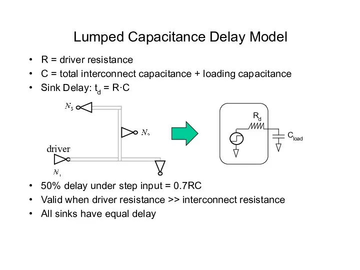
Lumped Capacitance Delay Model
R = driver resistance
C = total interconnect capacitance + loading
Lumped Capacitance Delay Model
R = driver resistance
C = total interconnect capacitance + loading
driver
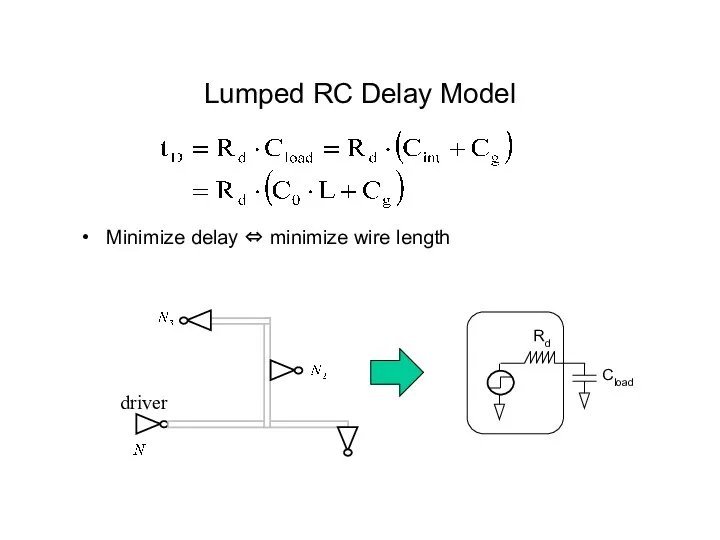
Lumped RC Delay Model
Minimize delay ⇔ minimize wire length
Rd
Cload
driver
Lumped RC Delay Model
Minimize delay ⇔ minimize wire length
Rd
Cload
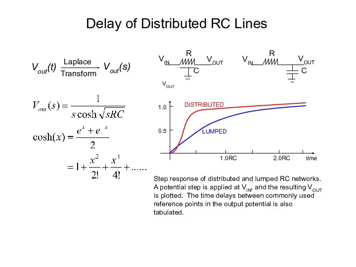
Delay of Distributed RC Lines
Vout(t)
Vout(s)
Laplace
Transform
R
VIN
VOUT
C
VOUT
VIN
R
C
0.5
1.0
VOUT
DISTRIBUTED
LUMPED
1.0RC
2.0RC
time
Step response of distributed and lumped RC networks.
A potential
Delay of Distributed RC Lines
Vout(t)
Vout(s)
Laplace
Transform
R
VIN
VOUT
C
VOUT
VIN
R
C
0.5
1.0
VOUT
DISTRIBUTED
LUMPED
1.0RC
2.0RC
time
Step response of distributed and lumped RC networks.
A potential
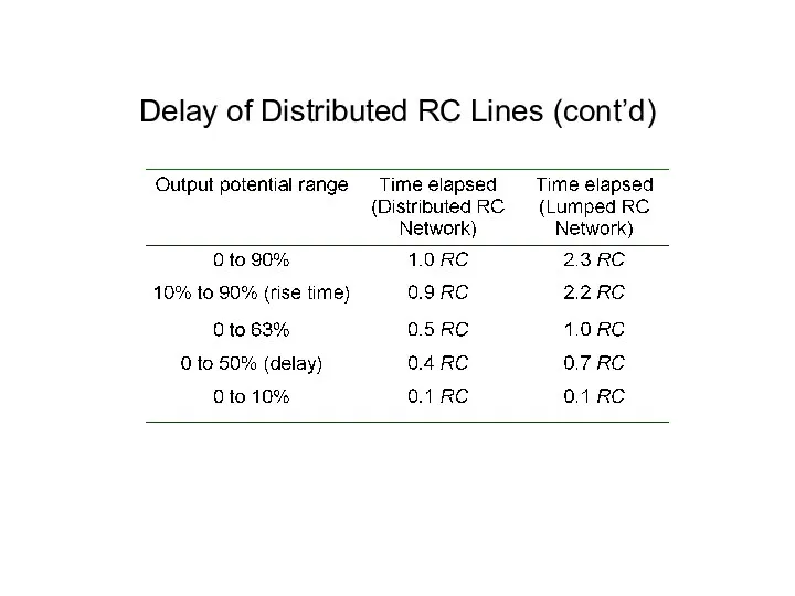
Delay of Distributed RC Lines (cont’d)
Delay of Distributed RC Lines (cont’d)
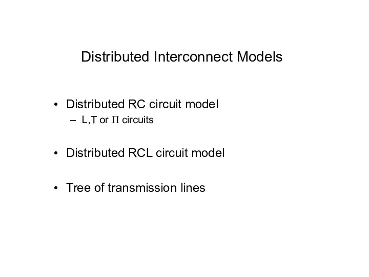
Distributed Interconnect Models
Distributed RC circuit model
L,T or Π circuits
Distributed RCL circuit model
Tree of
Distributed Interconnect Models
Distributed RC circuit model
L,T or Π circuits
Distributed RCL circuit model
Tree of
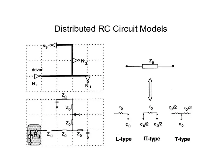
Distributed RC Circuit Models
Distributed RC Circuit Models
Distributed RLC Circuit Model
(without mutual inductance)
Distributed RLC Circuit Model
(without mutual inductance)
Delays of Complex Circuits under Unit Step Input
Circuits with monotonic response
Easy to define
Delays of Complex Circuits under Unit Step Input
Circuits with monotonic response
Easy to define
Delays of Complex Circuits under Unit Step Input (cont’d)
Circuits with non-monotonic response
Much more
Delays of Complex Circuits under Unit Step Input (cont’d)
Circuits with non-monotonic response
Much more
0.5
1
T50%
v(t)
t
t
v’(t)
median
of v’(t)
(T50%)
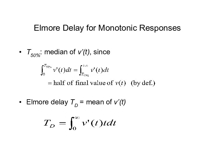
Elmore Delay for Monotonic Responses
Assumptions:
Unit step input
Monotone output response
Basic idea: use
0.5
1
T50%
v(t)
t
t
v’(t)
median
of v’(t)
(T50%)
Elmore Delay for Monotonic Responses
Assumptions:
Unit step input
Monotone output response
Basic idea: use
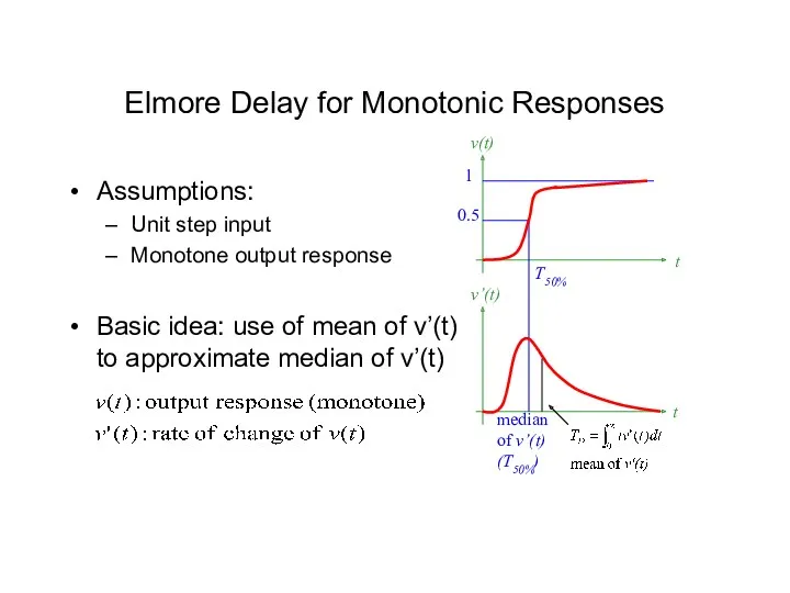
T50%: median of v’(t), since
Elmore delay TD = mean of v’(t)
Elmore Delay for
T50%: median of v’(t), since
Elmore delay TD = mean of v’(t)
Elmore Delay for
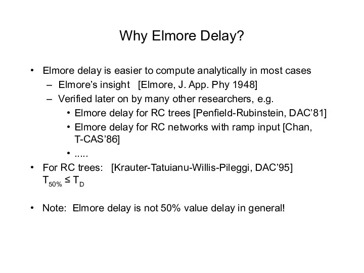
Why Elmore Delay?
Elmore delay is easier to compute analytically in most cases
Elmore’s insight [Elmore,
Why Elmore Delay?
Elmore delay is easier to compute analytically in most cases
Elmore’s insight [Elmore,
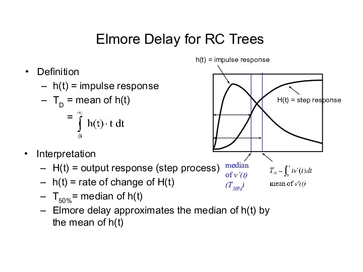
Elmore Delay for RC Trees
Definition
h(t) = impulse response
TD = mean of h(t)
=
Elmore Delay for RC Trees
Definition
h(t) = impulse response
TD = mean of h(t)
=
Elmore Delay of a RC Tree
[Rubinstein-Penfield-Horowitz, T-CAD’83]
Lemma:
Proof:
Apply impulse func. at t=0:
imin
i
current i→imin
Elmore Delay of a RC Tree
[Rubinstein-Penfield-Horowitz, T-CAD’83]
Lemma:
Proof:
Apply impulse func. at t=0:
imin
i
current i→imin
![Elmore Delay of a RC Tree [Rubinstein-Penfield-Horowitz, T-CAD’83] Lemma: Proof: Apply impulse func.](/_ipx/f_webp&q_80&fit_contain&s_1440x1080/imagesDir/jpg/383388/slide-21.jpg)
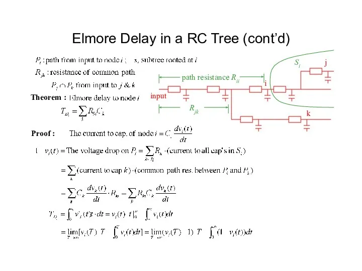
Elmore Delay in a RC Tree (cont’d)
input
i
k
j
Si
path resistance Rii
Rjk
Theorem :
Proof :
Elmore Delay in a RC Tree (cont’d)
input
i
k
j
Si
path resistance Rii
Rjk
Theorem :
Proof :
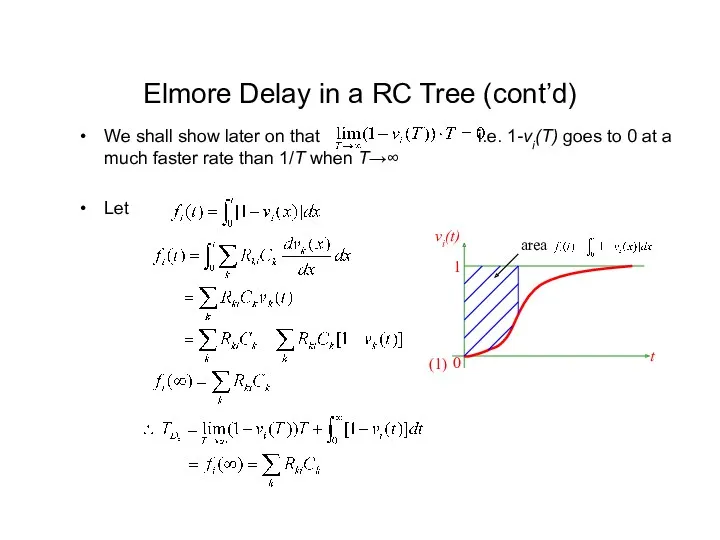
Elmore Delay in a RC Tree (cont’d)
We shall show later on that i.e.
Elmore Delay in a RC Tree (cont’d)
We shall show later on that i.e.
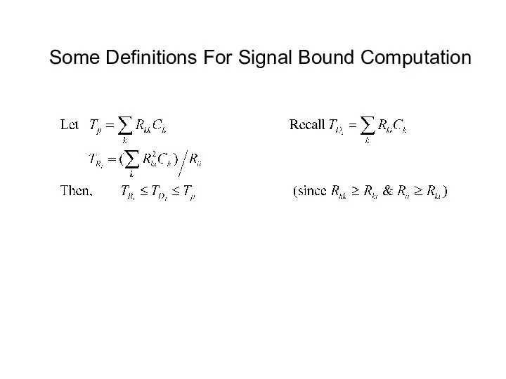
Some Definitions For Signal Bound Computation
Some Definitions For Signal Bound Computation
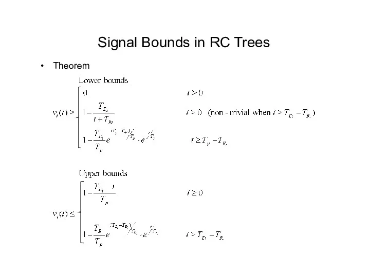
Signal Bounds in RC Trees
Theorem
Signal Bounds in RC Trees
Theorem
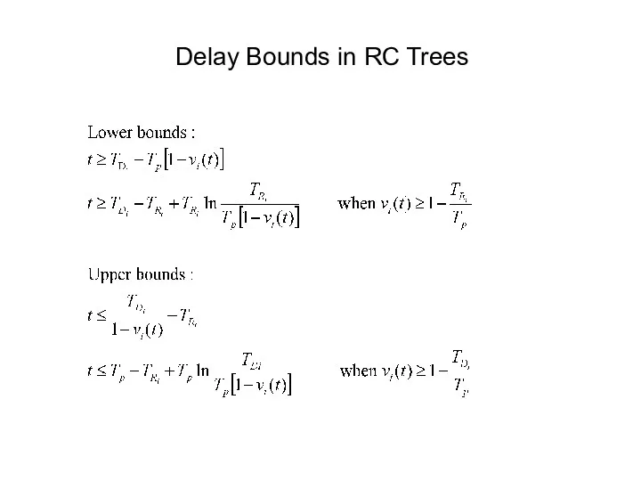
Delay Bounds in RC Trees
Delay Bounds in RC Trees
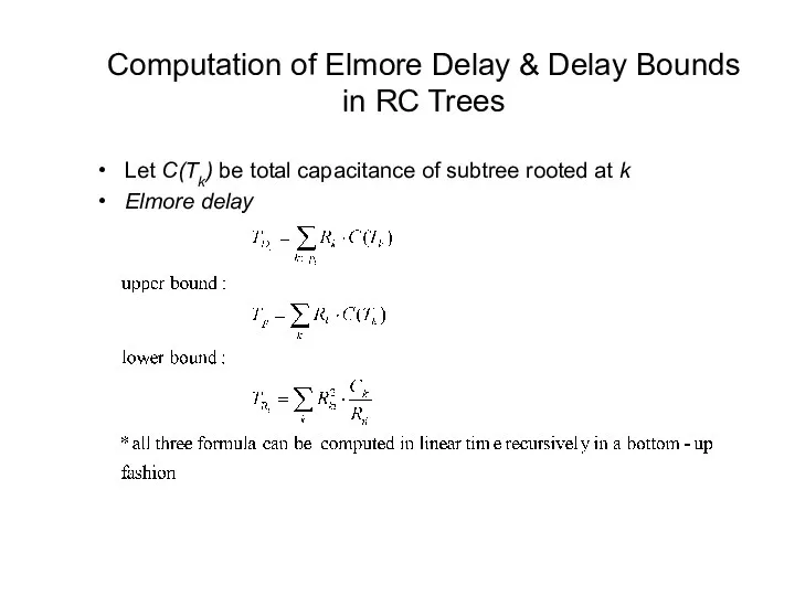
Computation of Elmore Delay & Delay Bounds in RC Trees
Let C(Tk) be total
Computation of Elmore Delay & Delay Bounds in RC Trees
Let C(Tk) be total
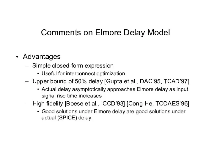
Comments on Elmore Delay Model
Advantages
Simple closed-form expression
Useful for interconnect optimization
Upper bound of 50%
Comments on Elmore Delay Model
Advantages
Simple closed-form expression
Useful for interconnect optimization
Upper bound of 50%
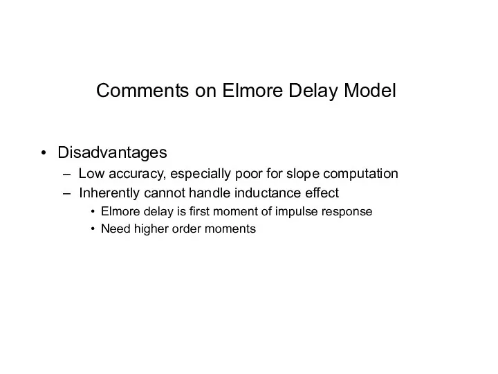
Comments on Elmore Delay Model
Disadvantages
Low accuracy, especially poor for slope computation
Inherently cannot handle
Comments on Elmore Delay Model
Disadvantages
Low accuracy, especially poor for slope computation
Inherently cannot handle
Chapter 7.2
Higher-order Delay Model
Chapter 7.2
Higher-order Delay Model
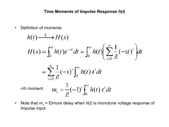
Time Moments of Impulse Response h(t)
Definition of moments
i-th moment
Note that m1 = Elmore
Time Moments of Impulse Response h(t)
Definition of moments
i-th moment
Note that m1 = Elmore
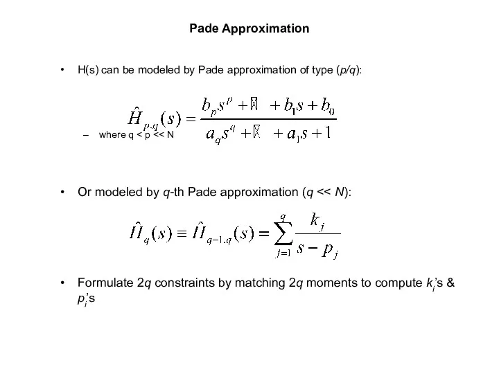
Pade Approximation
H(s) can be modeled by Pade approximation of type (p/q):
where q
Pade Approximation
H(s) can be modeled by Pade approximation of type (p/q):
where q
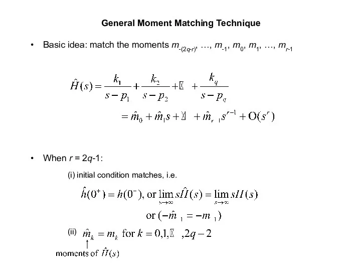
General Moment Matching Technique
Basic idea: match the moments m-(2q-r), …, m-1, m0, m1,
General Moment Matching Technique
Basic idea: match the moments m-(2q-r), …, m-1, m0, m1,
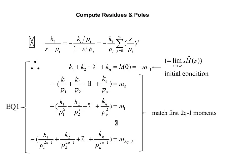
Compute Residues & Poles
match first 2q-1 moments
EQ1
Compute Residues & Poles
match first 2q-1 moments
EQ1
Basic Steps for Moment Matching
Step 1: Compute 2q moments m-1, m0, m1, …,
Basic Steps for Moment Matching
Step 1: Compute 2q moments m-1, m0, m1, …,
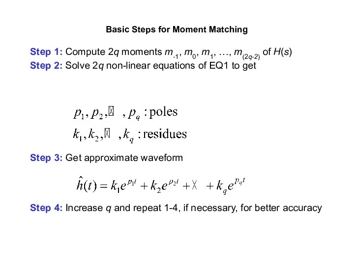
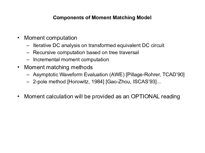
Components of Moment Matching Model
Moment computation
Iterative DC analysis on transformed equivalent DC circuit
Recursive
Components of Moment Matching Model
Moment computation
Iterative DC analysis on transformed equivalent DC circuit
Recursive
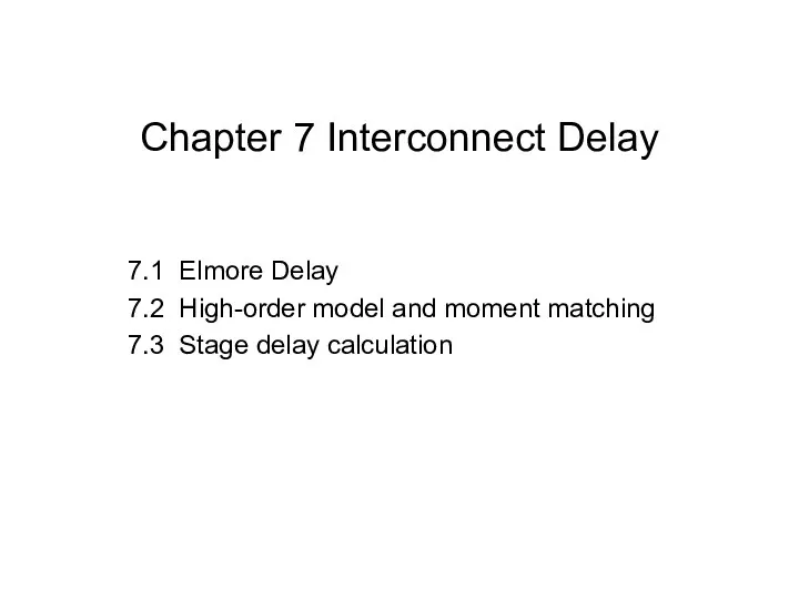
Chapter 7 Interconnect Delay
7.1 Elmore Delay
7.2 High-order model and moment matching
7.3 Stage delay
Chapter 7 Interconnect Delay
7.1 Elmore Delay
7.2 High-order model and moment matching
7.3 Stage delay
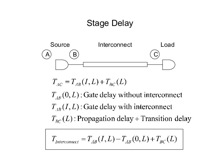
Stage Delay
A
B
C
Source
Interconnect
Load
Stage Delay
A
B
C
Source
Interconnect
Load
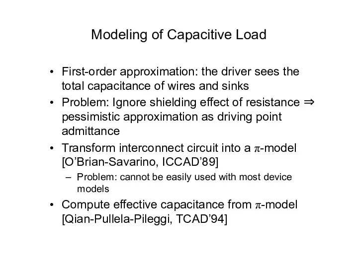
Modeling of Capacitive Load
First-order approximation: the driver sees the total capacitance of wires
Modeling of Capacitive Load
First-order approximation: the driver sees the total capacitance of wires
Π-Model
[O’Brian-Savarino, ICCAD’89]
Moment matching again!
Consider the first three moments of driving point admittance (moments
Π-Model
[O’Brian-Savarino, ICCAD’89]
Moment matching again!
Consider the first three moments of driving point admittance (moments
![Π-Model [O’Brian-Savarino, ICCAD’89] Moment matching again! Consider the first three moments of driving](/_ipx/f_webp&q_80&fit_contain&s_1440x1080/imagesDir/jpg/383388/slide-40.jpg)
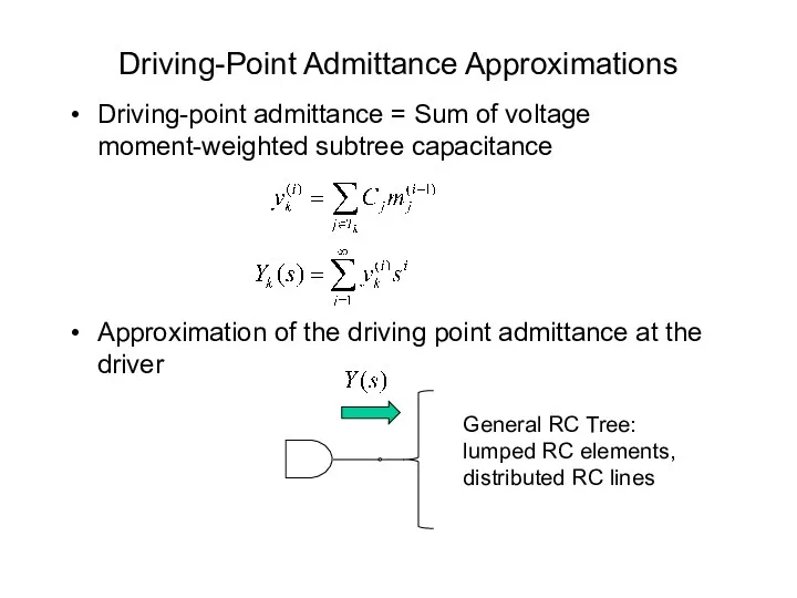
Driving-Point Admittance Approximations
Driving-point admittance = Sum of voltage moment-weighted subtree capacitance
Approximation of the
Driving-Point Admittance Approximations
Driving-point admittance = Sum of voltage moment-weighted subtree capacitance
Approximation of the
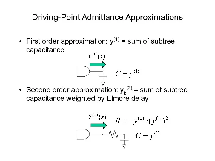
Driving-Point Admittance Approximations
First order approximation: y(1) = sum of subtree capacitance
Second order approximation:
Driving-Point Admittance Approximations
First order approximation: y(1) = sum of subtree capacitance
Second order approximation:
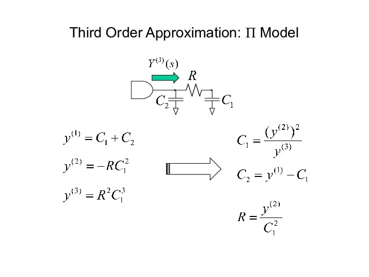
Third Order Approximation: Π Model
Third Order Approximation: Π Model
Current Moment Computation
Similar to the voltage moment computation
Iterative tree traversal:
O(n) run-time, O(n) storage
Bottom-up
Current Moment Computation
Similar to the voltage moment computation
Iterative tree traversal:
O(n) run-time, O(n) storage
Bottom-up
Bottom-Up Moment Computation
Maintain transfer function Hv~w(s) for sink w in subtree Tv, and
Bottom-Up Moment Computation
Maintain transfer function Hv~w(s) for sink w in subtree Tv, and
Current Moment Computation Rule #1
Current Moment Computation Rule #1
Current Moment Computation Rule #2
Current Moment Computation Rule #2
Current Moment Computation Rule #3
Current Moment Computation Rule #3
Current Moment Computation Rule #4
(Merging of Sub-trees)
B Branches
Current Moment Computation Rule #4
(Merging of Sub-trees)
B Branches
Example: Uniform Distributed RC Segment
Purely capacitive
Wide metal (distributive)
Narrow metal (distributive)
Narrow metal (lumped RC)
Wide
Example: Uniform Distributed RC Segment
Purely capacitive
Wide metal (distributive)
Narrow metal (distributive)
Narrow metal (lumped RC)
Wide
Why Effective Capacitance Model?
The π-model is incompatible with existing empirical device models
Mapping of
Why Effective Capacitance Model?
The π-model is incompatible with existing empirical device models
Mapping of
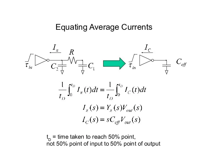
Equating Average Currents
tD = time taken to reach 50% point,
not 50% point
Equating Average Currents
tD = time taken to reach 50% point,
not 50% point
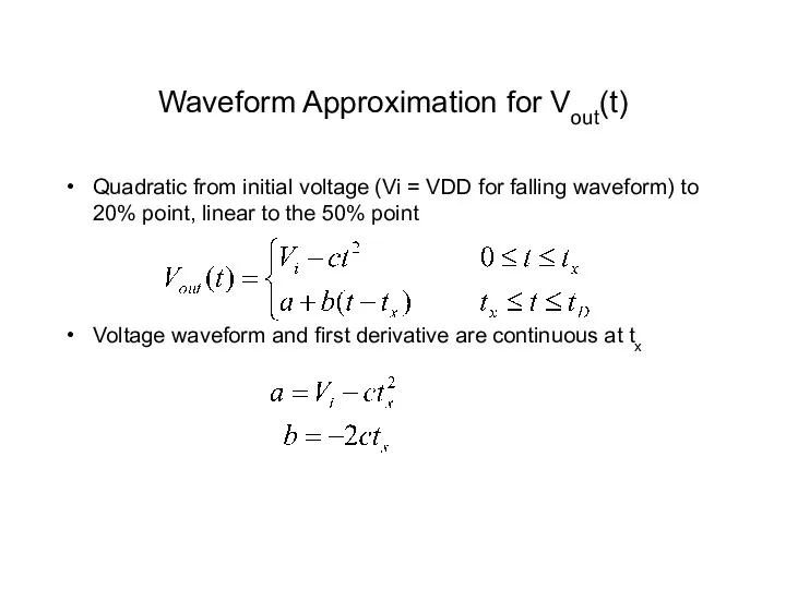
Waveform Approximation for Vout(t)
Quadratic from initial voltage (Vi = VDD for falling waveform)
Waveform Approximation for Vout(t)
Quadratic from initial voltage (Vi = VDD for falling waveform)
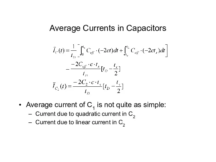
Average Currents in Capacitors
Average current of C1 is not quite as simple:
Current due
Average Currents in Capacitors
Average current of C1 is not quite as simple:
Current due
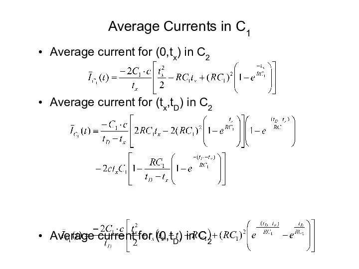
Average current for (0,tx) in C2
Average current for (tx,tD) in C2
Average current for
Average current for (0,tx) in C2
Average current for (tx,tD) in C2
Average current for
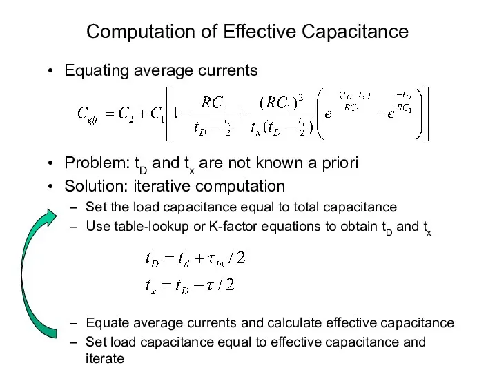
Computation of Effective Capacitance
Equating average currents
Problem: tD and tx are not known a
Computation of Effective Capacitance
Equating average currents
Problem: tD and tx are not known a
 Правила обслуговування аеронавігаційною інформацією
 Типы алгоритмов(Циклические)
 Алгоритмические языки и программирование
 Сервисы Google
 Программирование на языке Python. §62. Массивы
 Большой этнографический диктант
 Применение электронных ресурсов при проведении уроков информатики
 Delphi. Тест
 Типы алгоритмических структур с примерами
 Зміст навчання інформатики в середній загальноосвітній школі. (Лекція 2)
 Теория автоматов и формальных языков. Лекция 7
 Моделирование в электронных таблицах
 Метод излучательности (Radiosity)
 Искусственный интеллект
 Изменение формы представления информации
 Операционная система Windows
 Introduction to information systems. (Chapter 9)
 Решение задач на поиск выигрышной стратегии.
 Ветвления. Циклы (профориентация)
 Сетевая этика. Культура общения в сети. И зачем она нужна в Интернете
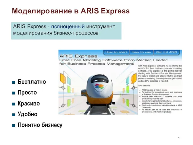 Моделирование в ARIS Express
 Безопасность в сети Интернет
 Основы организации UNIX. Занятие 02
 Растровая и векторная графика
 Личный кабинет подрядной организации
 Представление информации
 Урок по теме: Практическая работаПостроение диаграмм различных типов в табличном процессоре Open Office org Calc
 Прикладное программное обеспечение