- Introduction to CFX. Workshop 1 Mixing T-Junction

Содержание
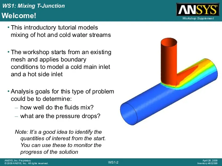
- 2. Welcome! This introductory tutorial models mixing of hot and cold water streams The workshop starts from
- 3. Pre-processing Goals Launch CFX-Pre from Workbench Use pre-defined materials Define the fluid models in a domain
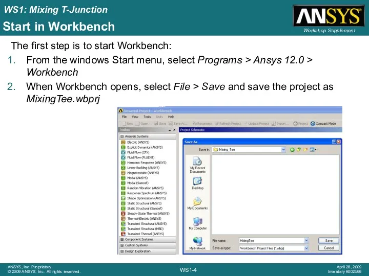
- 4. Start in Workbench The first step is to start Workbench: From the windows Start menu, select
- 5. Next, expand the Component Systems toolbox and drag a CFX analysis into the top left area
- 6. CFX-Pre GUI Overview Outline Tree New objects appear here as they are created Double-click to edit
- 7. CFX-Pre Mesh and Regions A domain named ‘Default Domain’ is automatically created from all 3-D regions
- 8. CFX-Pre – Domain settings The first step is to change the domain name to something more
- 9. CFX-Pre – Domain settings (continued) Double-click on the renamed domain junction Set the Material to Water.
- 10. CFX-Pre – Domain settings (continued) Click the Fluid Models tab In the Heat Transfer section, change
- 11. Boundary Conditions The next step is to create the boundary conditions. You will create a cold
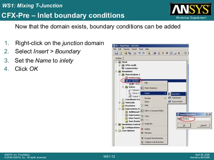
- 12. CFX-Pre – Inlet boundary conditions Now that the domain exists, boundary conditions can be added Right-click
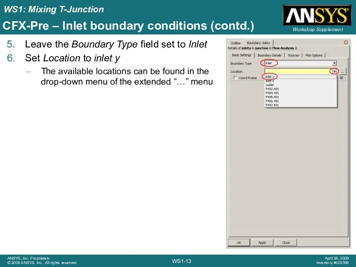
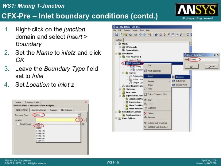
- 13. CFX-Pre – Inlet boundary conditions (contd.) Leave the Boundary Type field set to Inlet Set Location
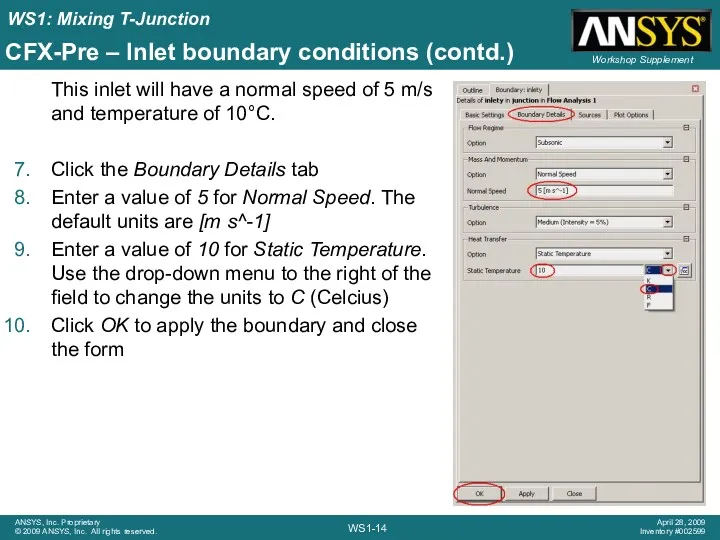
- 14. CFX-Pre – Inlet boundary conditions (contd.) This inlet will have a normal speed of 5 m/s
- 15. CFX-Pre – Inlet boundary conditions (contd.) Right-click on the junction domain and select Insert > Boundary
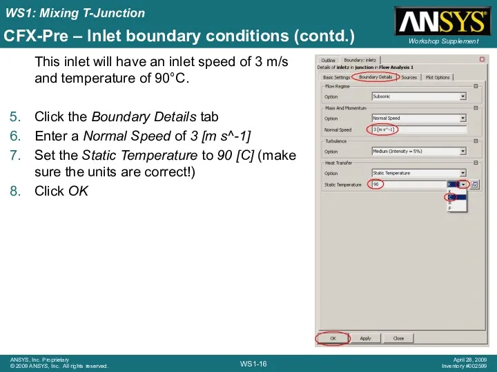
- 16. CFX-Pre – Inlet boundary conditions (contd.) This inlet will have an inlet speed of 3 m/s
- 17. CFX-Pre – Outlet boundary conditions Insert a boundary named outlet Set the Boundary Type to Outlet
- 18. CFX-Pre – Wall boundary conditions The default boundary condition (junction Default in this case) comprises of
- 19. Right-click on inlety and select Edit in Command Editor Close the Command Editor after taking a
- 20. Initialisation Automatic: This will use a previous solution if provided, otherwise the solver will generate an
- 21. Solver Control Double-click on Solver Control from the Outline tree The solver will stop after Max.
- 22. CFX-Pre – Monitor points Double-click Output Control from the Outline tree On the Output Control form,
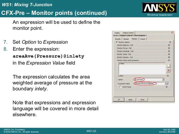
- 23. CFX-Pre – Monitor points (continued) An expression will be used to define the monitor point. Set
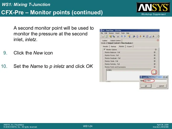
- 24. CFX-Pre – Monitor points (continued) A second monitor point will be used to monitor the pressure
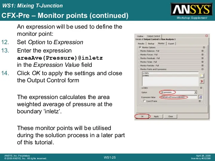
- 25. CFX-Pre – Monitor points (continued) An expression will be used to define the monitor point: Set
- 26. Solution Goals Launch CFX-Pre from Workbench. Use pre-defined materials. Define the fluid models in a domain.
- 27. Obtaining a solution Exit CFX-Pre When running in WB the CFX-Pre case will be saved automatically
- 28. Obtaining a solution (continued) The CFX Solver Manager will start with the simulation ready to run.
- 29. Post-processing Goals Launch CFX-Pre from Workbench. Use pre-defined materials. Define the fluid models in a domain.
- 30. Launching CFD-Post Exit the CFX Solver Manager Save the project Double click Results to launch CFD-Post
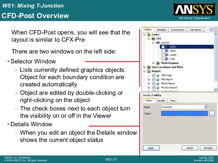
- 31. CFD-Post Overview Selector Window Lists currently defined graphics objects. Object for each boundary condition are created
- 32. CFD-Post – Manipulating the view When the results are loaded, CFD-Post displays the outline (wireframe) of
- 33. CFD-Post – Temperature contour plot In the first step, you will plot contours of temperature on
- 34. CFD-Post – Temperature contour plot (contd.) Set the Variable to Temperature The drop-down menu provides a
- 35. CFD-Post - Temperature contour plot (contd.) A temperature contour plot on the walls should now be
- 36. CFD-Post Location: Points, Lines, Planes, Surfaces, Volumes Vector Plots Contour Plots Streamline Plots Particle Track (if
- 37. CFD-Post – Creating a plane at x = 0 First, hide the previously created contour plot,
- 38. CFD-Post – Creating a plane at x = 0 (contd.) Set Method to YZ Plane Leave
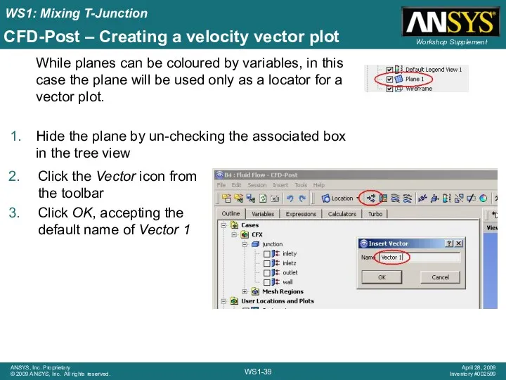
- 39. CFD-Post – Creating a velocity vector plot While planes can be coloured by variables, in this
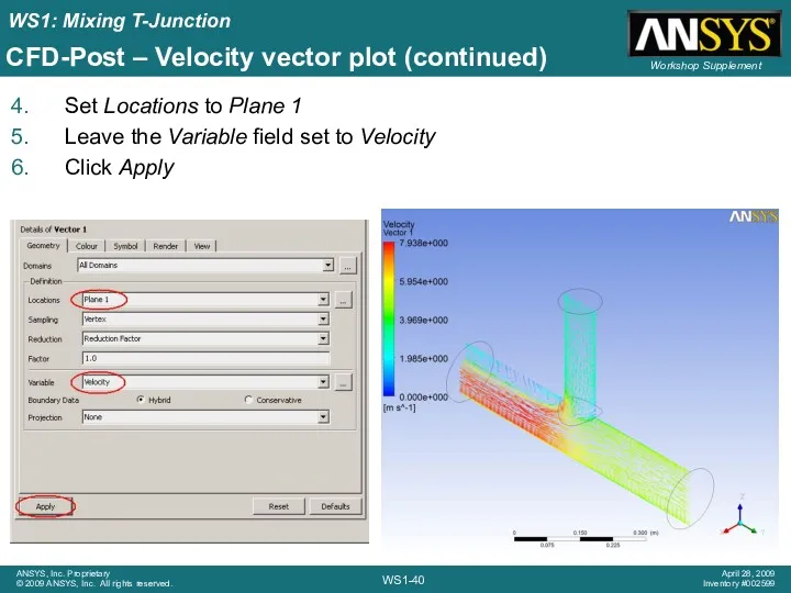
- 40. CFD-Post – Velocity vector plot (continued) Set Locations to Plane 1 Leave the Variable field set
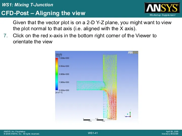
- 41. CFD-Post – Aligning the view Given that the vector plot is on a 2-D Y-Z plane,
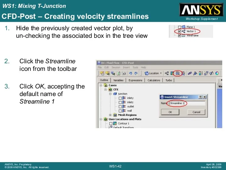
- 42. CFD-Post – Creating velocity streamlines Hide the previously created vector plot, by un-checking the associated box
- 43. CFD-Post – Velocity streamlines (continued) In the Start From field, select both inlety and inletz. Use
- 44. CFD-Post – Velocity streamlines (continued) Click the Symbol tab Change the Stream Type to Ribbon Click
- 45. CFD-Post – Creating a velocity isosurface Hide the previously created streamlines, by un-checking the associated box
- 46. CFD-Post – Velocity isosurface (continued) Set the Variable to Velocity (magnitude used in this context) Enter
- 48. Скачать презентацию
Welcome!
This introductory tutorial models mixing of hot and cold water streams
The
Welcome!
This introductory tutorial models mixing of hot and cold water streams
The
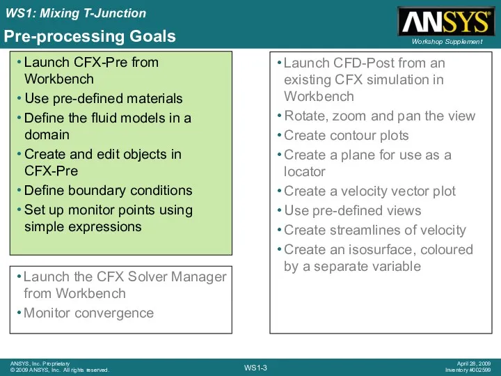
Pre-processing Goals
Launch CFX-Pre from Workbench
Use pre-defined materials
Define the fluid models in
Pre-processing Goals
Launch CFX-Pre from Workbench
Use pre-defined materials
Define the fluid models in
Start in Workbench
The first step is to start Workbench:
From the windows
Start in Workbench
The first step is to start Workbench:
From the windows
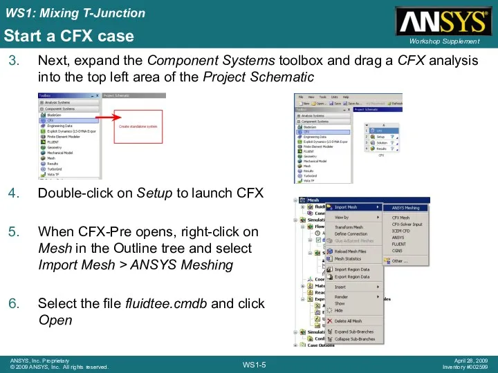
Next, expand the Component Systems toolbox and drag a CFX analysis
Next, expand the Component Systems toolbox and drag a CFX analysis
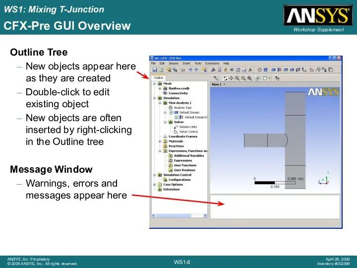
CFX-Pre GUI Overview
Outline Tree
New objects appear here as they are created
Double-click
CFX-Pre GUI Overview
Outline Tree
New objects appear here as they are created
Double-click
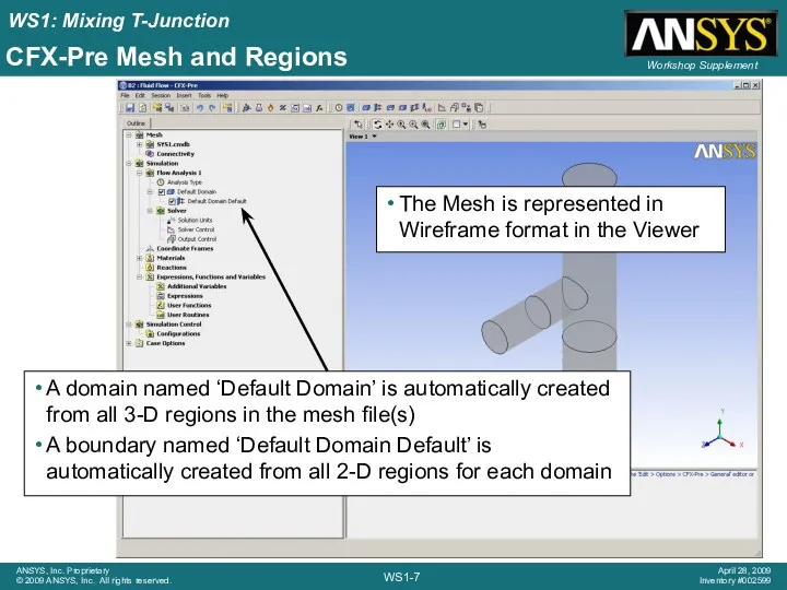
CFX-Pre Mesh and Regions
A domain named ‘Default Domain’ is automatically created
CFX-Pre Mesh and Regions
A domain named ‘Default Domain’ is automatically created
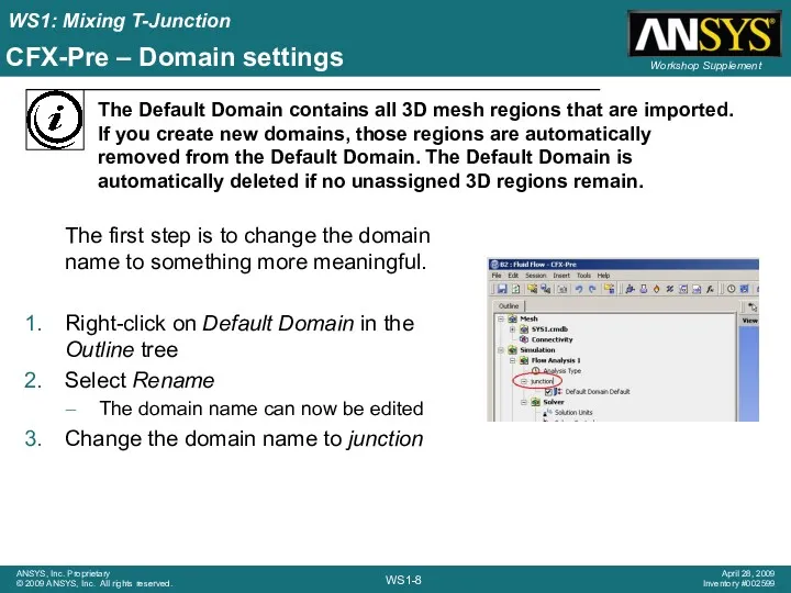
CFX-Pre – Domain settings
The first step is to change the domain
CFX-Pre – Domain settings
The first step is to change the domain
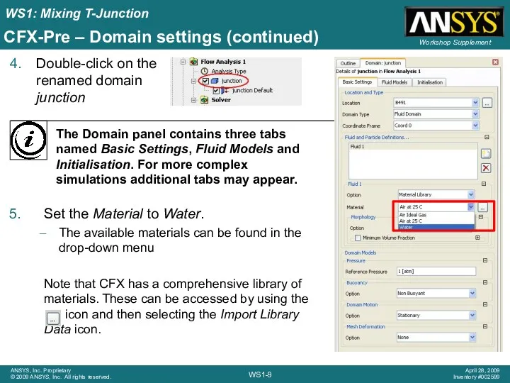
CFX-Pre – Domain settings (continued)
Double-click on the renamed domain junction
Set the
CFX-Pre – Domain settings (continued)
Double-click on the renamed domain junction
Set the

CFX-Pre – Domain settings (continued)
Click the Fluid Models tab
In the Heat
CFX-Pre – Domain settings (continued)
Click the Fluid Models tab
In the Heat
Boundary Conditions
The next step is to create the boundary conditions. You
Boundary Conditions
The next step is to create the boundary conditions. You
CFX-Pre – Inlet boundary conditions
Now that the domain exists, boundary conditions
CFX-Pre – Inlet boundary conditions
Now that the domain exists, boundary conditions
CFX-Pre – Inlet boundary conditions (contd.)
Leave the Boundary Type field set
CFX-Pre – Inlet boundary conditions (contd.)
Leave the Boundary Type field set
CFX-Pre – Inlet boundary conditions (contd.)
This inlet will have a normal
CFX-Pre – Inlet boundary conditions (contd.)
This inlet will have a normal
CFX-Pre – Inlet boundary conditions (contd.)
Right-click on the junction domain and
CFX-Pre – Inlet boundary conditions (contd.)
Right-click on the junction domain and
CFX-Pre – Inlet boundary conditions (contd.)
This inlet will have an inlet
CFX-Pre – Inlet boundary conditions (contd.)
This inlet will have an inlet
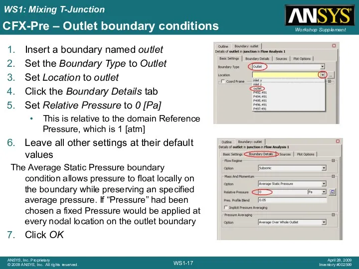
CFX-Pre – Outlet boundary conditions
Insert a boundary named outlet
Set the Boundary
CFX-Pre – Outlet boundary conditions
Insert a boundary named outlet
Set the Boundary
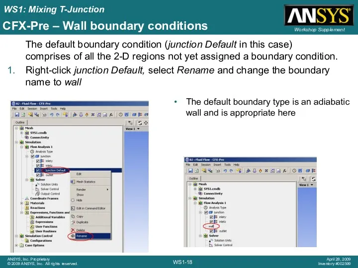
CFX-Pre – Wall boundary conditions
The default boundary condition (junction Default in
CFX-Pre – Wall boundary conditions
The default boundary condition (junction Default in
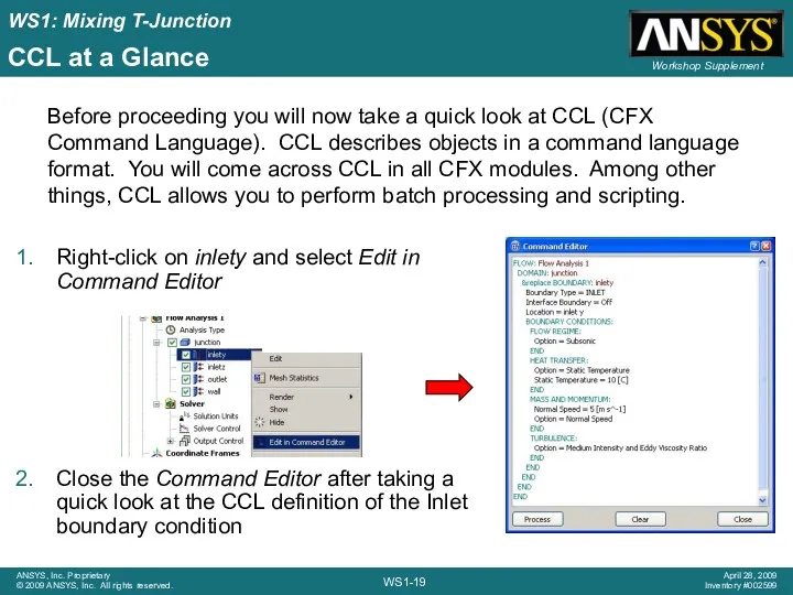
Right-click on inlety and select Edit in Command Editor
Close the Command
Right-click on inlety and select Edit in Command Editor
Close the Command
Initialisation
Automatic: This will use a previous solution if provided, otherwise the
Initialisation
Automatic: This will use a previous solution if provided, otherwise the
Solver Control
Double-click on Solver Control from the Outline tree
The solver will
Solver Control
Double-click on Solver Control from the Outline tree
The solver will
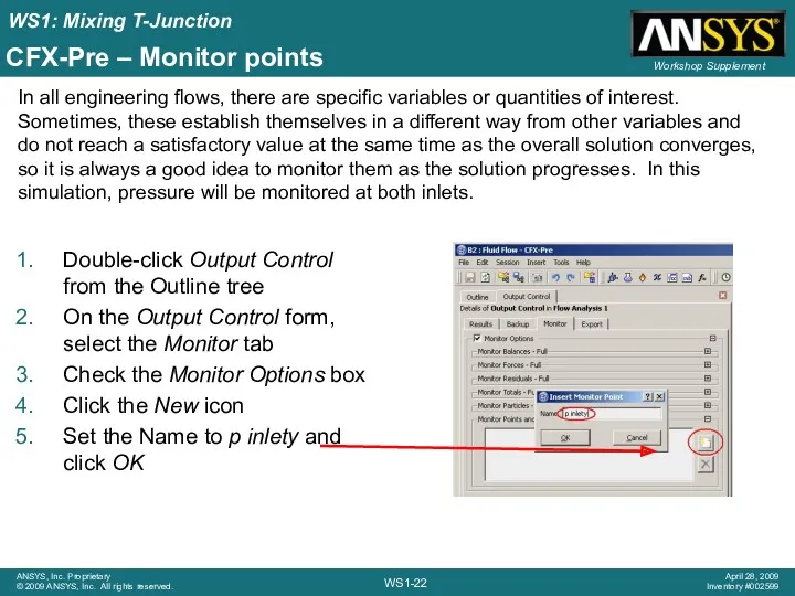
CFX-Pre – Monitor points
Double-click Output Control from the Outline tree
On the
CFX-Pre – Monitor points
Double-click Output Control from the Outline tree
On the
CFX-Pre – Monitor points (continued)
An expression will be used to define
CFX-Pre – Monitor points (continued)
An expression will be used to define
CFX-Pre – Monitor points (continued)
A second monitor point will be used
CFX-Pre – Monitor points (continued)
A second monitor point will be used
CFX-Pre – Monitor points (continued)
An expression will be used to define
CFX-Pre – Monitor points (continued)
An expression will be used to define
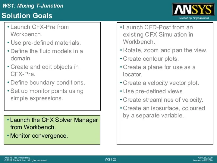
Solution Goals
Launch CFX-Pre from Workbench.
Use pre-defined materials.
Define the fluid models in
Solution Goals
Launch CFX-Pre from Workbench.
Use pre-defined materials.
Define the fluid models in
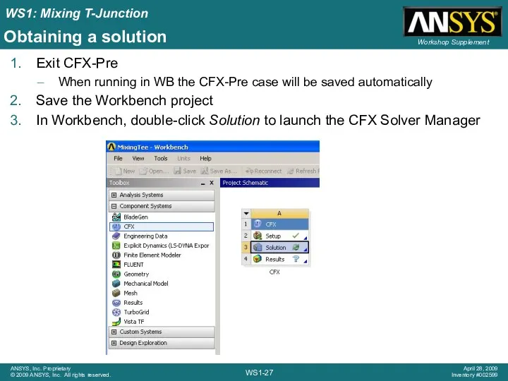
Obtaining a solution
Exit CFX-Pre
When running in WB the CFX-Pre case will
Obtaining a solution
Exit CFX-Pre
When running in WB the CFX-Pre case will
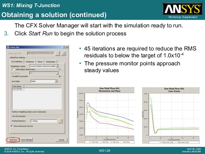
Obtaining a solution (continued)
The CFX Solver Manager will start with the
Obtaining a solution (continued)
The CFX Solver Manager will start with the
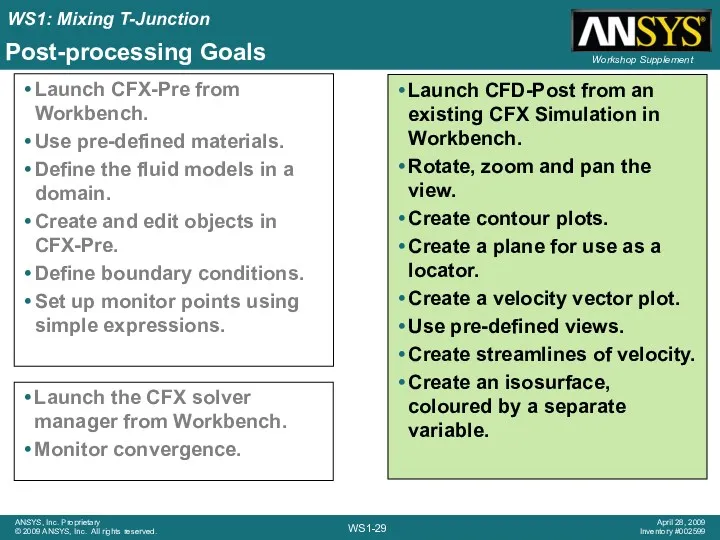
Post-processing Goals
Launch CFX-Pre from Workbench.
Use pre-defined materials.
Define the fluid models in
Post-processing Goals
Launch CFX-Pre from Workbench.
Use pre-defined materials.
Define the fluid models in
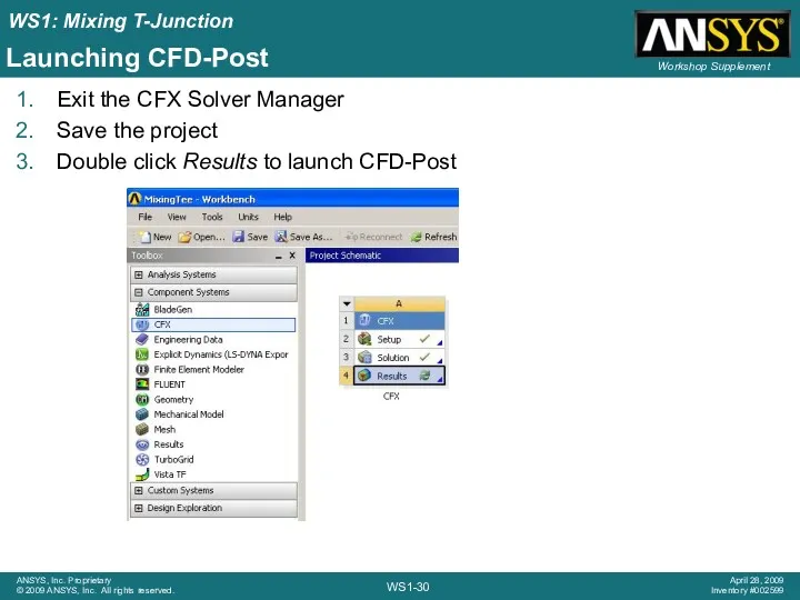
Launching CFD-Post
Exit the CFX Solver Manager
Save the project
Double click Results to
Launching CFD-Post
Exit the CFX Solver Manager
Save the project
Double click Results to
CFD-Post Overview
Selector Window
Lists currently defined graphics objects. Object for each boundary
CFD-Post Overview
Selector Window
Lists currently defined graphics objects. Object for each boundary
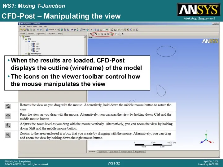
CFD-Post – Manipulating the view
When the results are loaded, CFD-Post displays
CFD-Post – Manipulating the view
When the results are loaded, CFD-Post displays
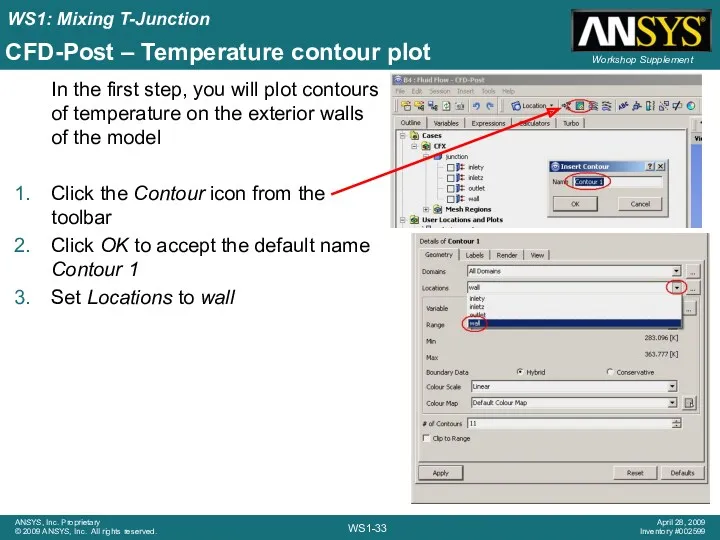
CFD-Post – Temperature contour plot
In the first step, you will plot
CFD-Post – Temperature contour plot
In the first step, you will plot
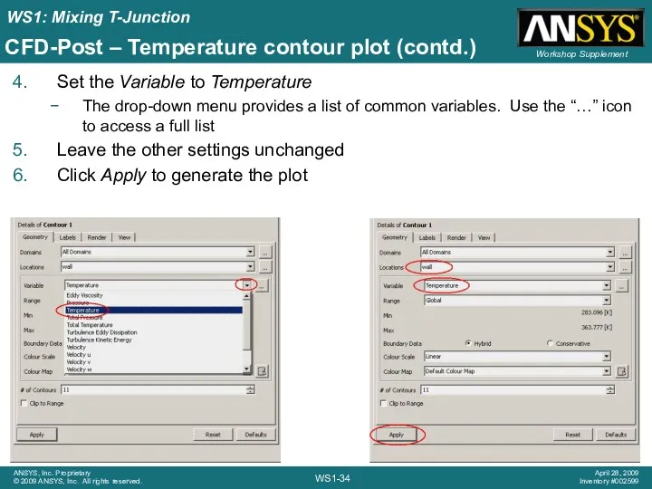
CFD-Post – Temperature contour plot (contd.)
Set the Variable to Temperature
The drop-down
CFD-Post – Temperature contour plot (contd.)
Set the Variable to Temperature
The drop-down
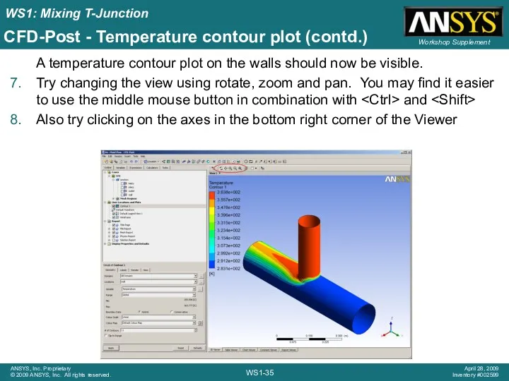
CFD-Post - Temperature contour plot (contd.)
A temperature contour plot on the
CFD-Post - Temperature contour plot (contd.)
A temperature contour plot on the
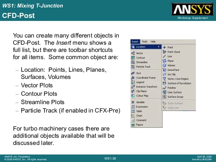
CFD-Post
Location: Points, Lines, Planes, Surfaces, Volumes
Vector Plots
Contour Plots
Streamline Plots
Particle Track (if
CFD-Post
Location: Points, Lines, Planes, Surfaces, Volumes
Vector Plots
Contour Plots
Streamline Plots
Particle Track (if
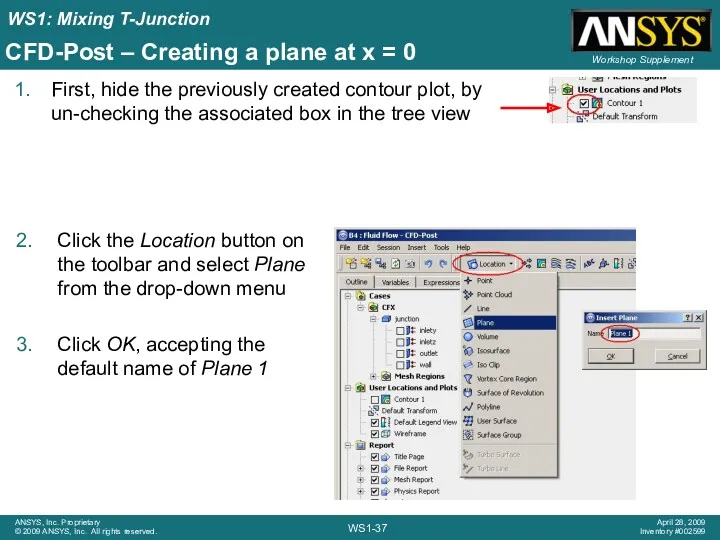
CFD-Post – Creating a plane at x = 0
First, hide the
CFD-Post – Creating a plane at x = 0
First, hide the
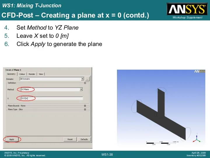
CFD-Post – Creating a plane at x = 0 (contd.)
Set Method
CFD-Post – Creating a plane at x = 0 (contd.)
Set Method
CFD-Post – Creating a velocity vector plot
While planes can be coloured
CFD-Post – Creating a velocity vector plot
While planes can be coloured
CFD-Post – Velocity vector plot (continued)
Set Locations to Plane 1
Leave the
CFD-Post – Velocity vector plot (continued)
Set Locations to Plane 1
Leave the
CFD-Post – Aligning the view
Given that the vector plot is on
CFD-Post – Aligning the view
Given that the vector plot is on
CFD-Post – Creating velocity streamlines
Hide the previously created vector plot, by
CFD-Post – Creating velocity streamlines
Hide the previously created vector plot, by
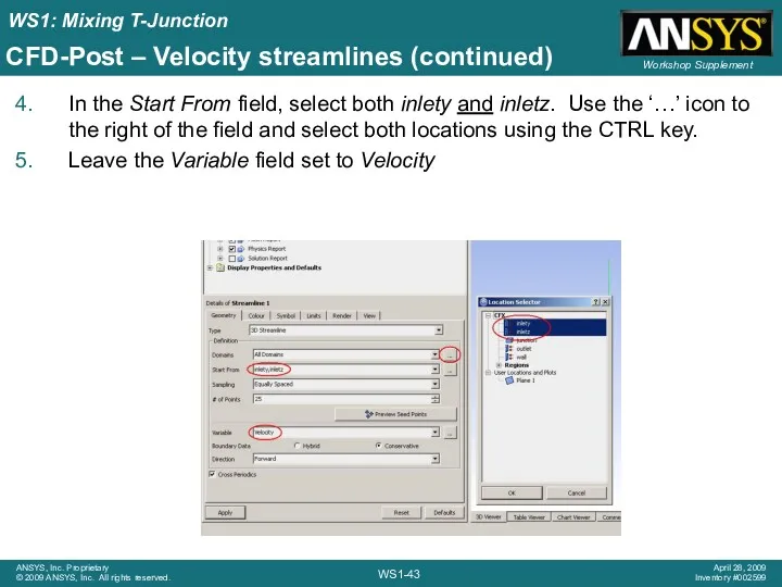
CFD-Post – Velocity streamlines (continued)
In the Start From field, select both
CFD-Post – Velocity streamlines (continued)
In the Start From field, select both
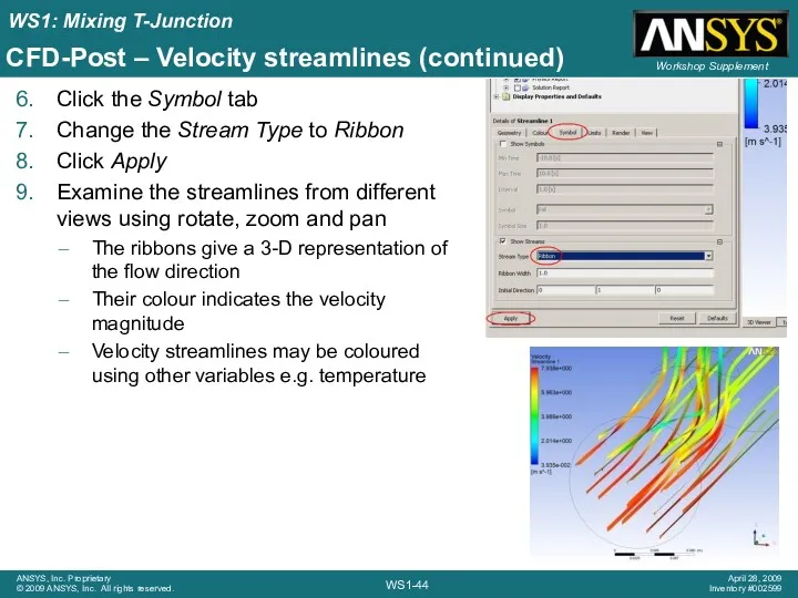
CFD-Post – Velocity streamlines (continued)
Click the Symbol tab
Change the Stream Type
CFD-Post – Velocity streamlines (continued)
Click the Symbol tab
Change the Stream Type
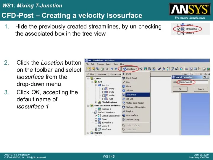
CFD-Post – Creating a velocity isosurface
Hide the previously created streamlines, by
CFD-Post – Creating a velocity isosurface
Hide the previously created streamlines, by
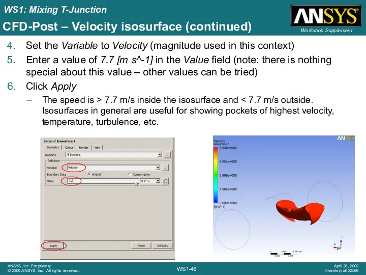
CFD-Post – Velocity isosurface (continued)
Set the Variable to Velocity (magnitude used
CFD-Post – Velocity isosurface (continued)
Set the Variable to Velocity (magnitude used
 Техзадание к сайту
 Моделирование систем. Лекция 1
 Офисные информационные технологии
 Учет библиотечной работы. Учетная документация. Онлайн-семинар
 Апгрейд телефонов для школьников
 Idena. The first human-centric blockchain
 PR on the Internet
 Одномерный массив
 SAP HANA – платформа для бизнеса в реальном времени
 Количественные методы исследований (SPSS) DATA ANALYSIS
 Компьютерные сети. Виды локальных сетей. Топология сети
 АРМ Реестр государственных и муниципальных услуг
 Konsep Dasar Algoritma
 Аналіз систем, які працюють за дисципліною обслуговування з очікуванням
 Составные типы данных
 НОУ Клуб знатоков. Секция информатики Инфознайка
 Директивы препроцессора
 Информационные системы и программирование
 Организация защиты персональных данных в корпорации RHANA
 Обучение компьютерной грамотности граждан старшего возраста на базе программы Азбука Интернета
 Электронная почта e-mail
 Курсовий проект з дисципліни Програмування на тему: напівпровідникові прилади
 Информационная безопасность в цифровой реальности
 Запуск Android приложения
 Диаграмма классов языка UML 2 (Лекция 3)
 Операторы в языке Си. (Лекция 5)
 Создание игры на движке Construct 2
 Модель параллельного программирования. Лекция 2