- Introduction to CFX. Workshop 3 Room Temperature Study

Содержание
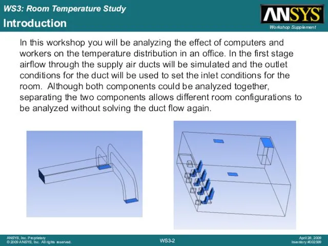
- 2. Introduction In this workshop you will be analyzing the effect of computers and workers on the
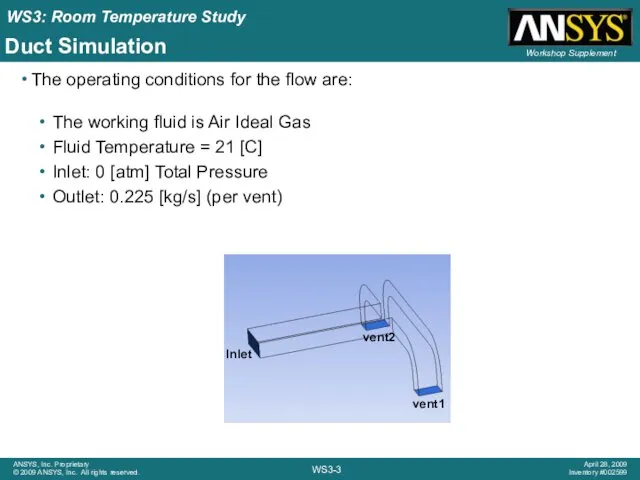
- 3. Duct Simulation The operating conditions for the flow are: The working fluid is Air Ideal Gas
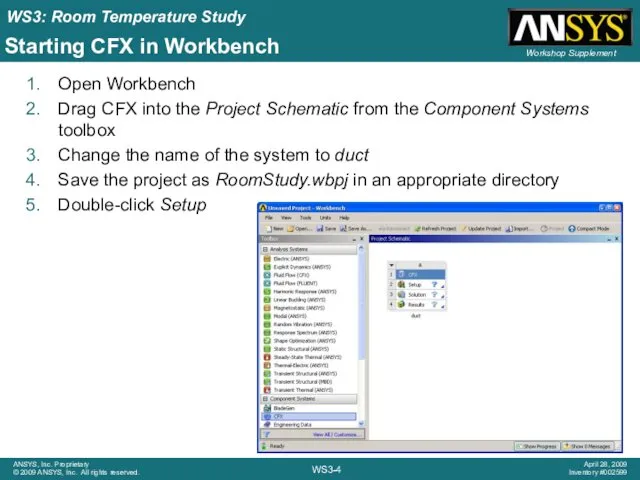
- 4. Starting CFX in Workbench Open Workbench Drag CFX into the Project Schematic from the Component Systems
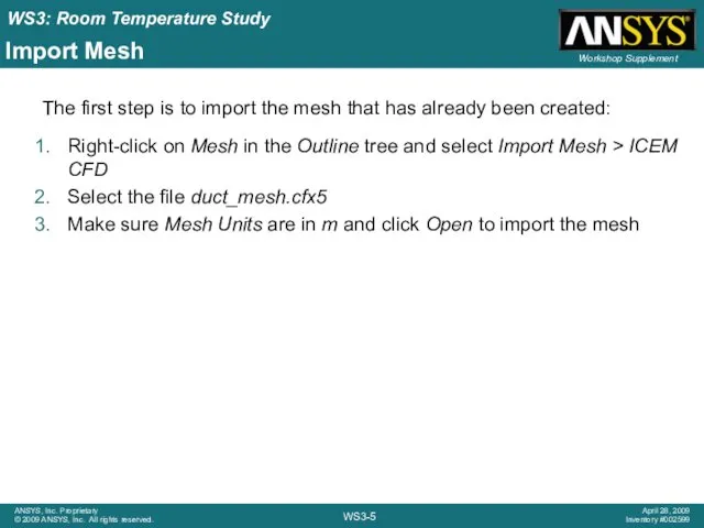
- 5. Import Mesh Right-click on Mesh in the Outline tree and select Import Mesh > ICEM CFD
- 6. Create Domain Double-click on Default Domain in the Outline tree to edit the domain On the
- 7. Create Boundary Conditions INLET Boundary Condition Name: INLET Boundary Type: Inlet Location: INLET Mass and Momentum
- 8. Solver Control Double click on Solver Control from the Outline tree Enable the Conservation Target toggle
- 9. Monitor Point Double click on Output Control from the Outline tree Switch to the Monitor tab
- 10. Monitor Point In the Expression Value field, type in: areaAve(Velocity w)@VENT1 Click OK to create the
- 11. Write Solver File Close CFX-Pre to return to Project window Save the project Right-click on Solution
- 12. Examine the residual plots for Momentum and Mass and Turbulence Examine the User Points plot When
- 13. CFD-Post Select File > Export Change the file name to vent1.csv Use the browse icon to
- 14. Operating Conditions The working fluid is Air Ideal Gas Computer Monitor Temperature = 30 [C] Computer
- 15. Starting Room Simulation in Workbench Drag CFX into the Project Schematic from the Component Systems toolbox
- 16. Import Mesh Right-click on Mesh in the Outline tree and select Import Mesh > ICEM CFD
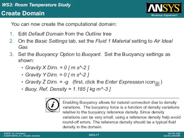
- 17. Create Domain Edit Default Domain from the Outline tree On the Basic Settings tab, set the
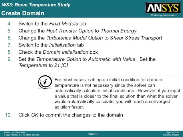
- 18. Create Domain Switch to the Fluid Models tab Change the Heat Transfer Option to Thermal Energy
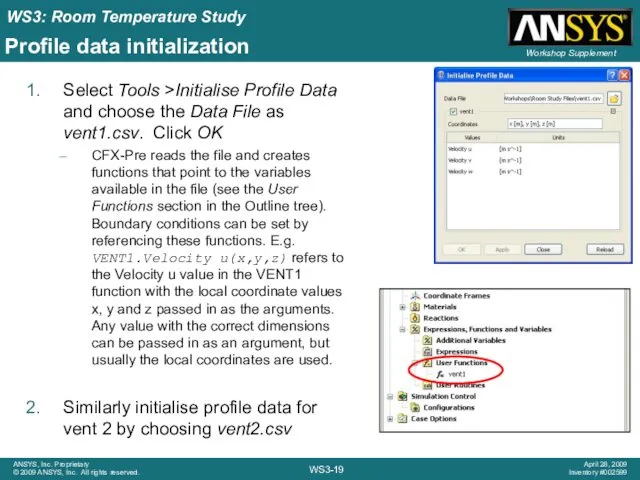
- 19. Profile data initialization Select Tools >Initialise Profile Data and choose the Data File as vent1.csv. Click
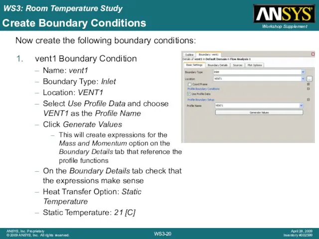
- 20. Create Boundary Conditions vent1 Boundary Condition Name: vent1 Boundary Type: Inlet Location: VENT1 Select Use Profile
- 21. vent2 Boundary Condition Name: vent2 Boundary Type: Inlet Location: VENT2 Select Use Profile Data and choose
- 22. outlet Boundary Condition Name: outlet Boundary Type: Opening Location: OUTLET Mass and Momentum Option: Opening Pres.
- 23. computerVent Boundary Condition Name: computerVent Boundary Type: Inlet Location: COMPUTER1VENT, COMPUTER2VENT, COMPUTER3VENT, COMPUTER4VENT Mass and Momentum
- 24. computerIntake Boundary Condition Name: computerIntake Boundary Type: Outlet Location: COMPUTER1INTAKE, COMPUTER2INTAKE, COMPUTER3INTAKE, COMPUTER4INTAKE Mass and Momentum
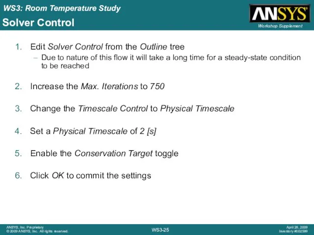
- 25. Solver Control Edit Solver Control from the Outline tree Due to nature of this flow it
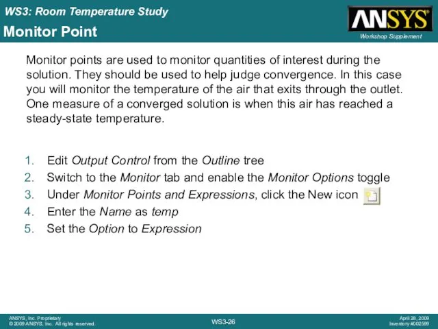
- 26. Monitor Point Edit Output Control from the Outline tree Switch to the Monitor tab and enable
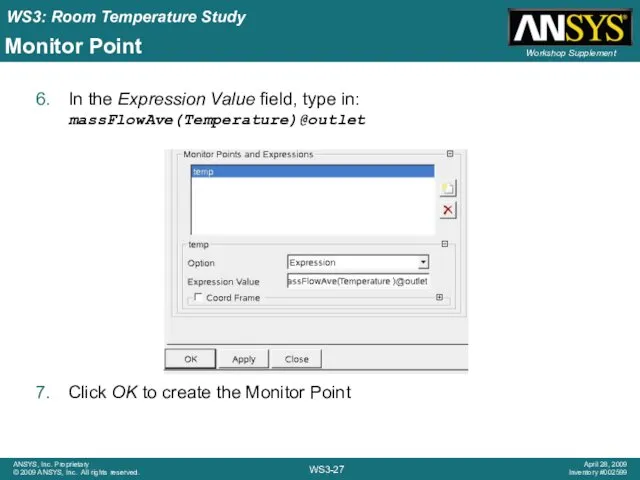
- 27. Monitor Point In the Expression Value field, type in: massFlowAve(Temperature)@outlet Click OK to create the Monitor
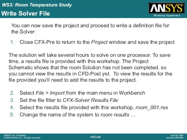
- 28. Write Solver File Close CFX-Pre to return to the Project window and save the project Select
- 29. Project Schematic
- 30. CFX Solver Manager Right-click on Solution in the room results system and select Display Monitors Examine
- 31. Residual and Monitor plot Residual plot Monitor points
- 32. CFX Solver Manager Check the Domain Imbalances at the end of the .out file for each
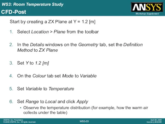
- 33. CFD-Post Select Location > Plane from the toolbar In the Details windows on the Geometry tab,
- 34. CFD-Post ZX Plane at Y = 2 [m] ZX Plane at Y = 5.1 [m] XY
- 35. CFD-Post Click Insert > Vector from the main menu In the Details windows on the Geometry
- 37. Скачать презентацию
Introduction
In this workshop you will be analyzing the effect of computers
Introduction
In this workshop you will be analyzing the effect of computers
Duct Simulation
The operating conditions for the flow are:
The working fluid is
Duct Simulation
The operating conditions for the flow are:
The working fluid is
Starting CFX in Workbench
Open Workbench
Drag CFX into the Project Schematic from
Starting CFX in Workbench
Open Workbench
Drag CFX into the Project Schematic from
Import Mesh
Right-click on Mesh in the Outline tree and select Import
Import Mesh
Right-click on Mesh in the Outline tree and select Import
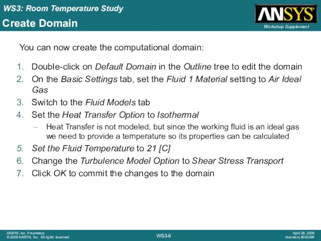
Create Domain
Double-click on Default Domain in the Outline tree to edit
Create Domain
Double-click on Default Domain in the Outline tree to edit
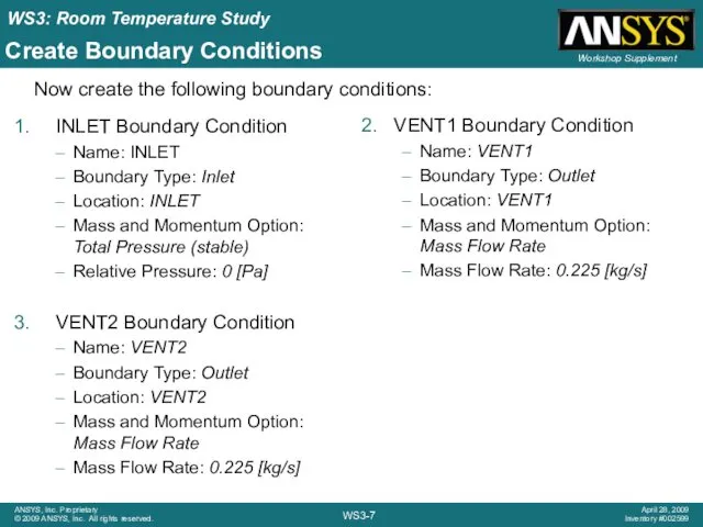
Create Boundary Conditions
INLET Boundary Condition
Name: INLET
Boundary Type: Inlet
Location: INLET
Mass and Momentum
Create Boundary Conditions
INLET Boundary Condition
Name: INLET
Boundary Type: Inlet
Location: INLET
Mass and Momentum
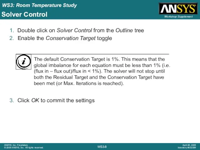
Solver Control
Double click on Solver Control from the Outline tree
Enable the
Solver Control
Double click on Solver Control from the Outline tree
Enable the
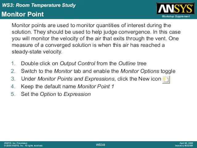
Monitor Point
Double click on Output Control from the Outline tree
Switch to
Monitor Point
Double click on Output Control from the Outline tree
Switch to

Monitor Point
In the Expression Value field, type in:
areaAve(Velocity w)@VENT1
Click OK to
Monitor Point
In the Expression Value field, type in:
areaAve(Velocity w)@VENT1
Click OK to
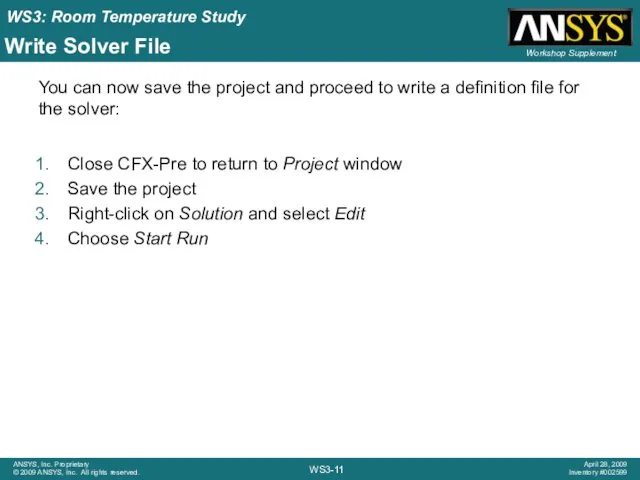
Write Solver File
Close CFX-Pre to return to Project window
Save the project
Right-click
Write Solver File
Close CFX-Pre to return to Project window
Save the project
Right-click
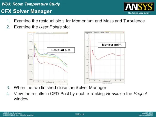
Examine the residual plots for Momentum and Mass and Turbulence
Examine the
Examine the residual plots for Momentum and Mass and Turbulence
Examine the
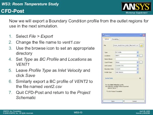
CFD-Post
Select File > Export
Change the file name to vent1.csv
Use the browse
CFD-Post
Select File > Export
Change the file name to vent1.csv
Use the browse

Operating Conditions
The working fluid is Air Ideal Gas
Computer Monitor Temperature =
Operating Conditions
The working fluid is Air Ideal Gas
Computer Monitor Temperature =

Starting Room Simulation in Workbench
Drag CFX into the Project Schematic from
Starting Room Simulation in Workbench
Drag CFX into the Project Schematic from
Import Mesh
Right-click on Mesh in the Outline tree and select Import
Import Mesh
Right-click on Mesh in the Outline tree and select Import
Create Domain
Edit Default Domain from the Outline tree
On the Basic Settings
Create Domain
Edit Default Domain from the Outline tree
On the Basic Settings
Create Domain
Switch to the Fluid Models tab
Change the Heat Transfer Option
Create Domain
Switch to the Fluid Models tab
Change the Heat Transfer Option
Profile data initialization
Select Tools >Initialise Profile Data and choose the Data
Profile data initialization
Select Tools >Initialise Profile Data and choose the Data
Create Boundary Conditions
vent1 Boundary Condition
Name: vent1
Boundary Type: Inlet
Location: VENT1
Select Use Profile
Create Boundary Conditions
vent1 Boundary Condition
Name: vent1
Boundary Type: Inlet
Location: VENT1
Select Use Profile
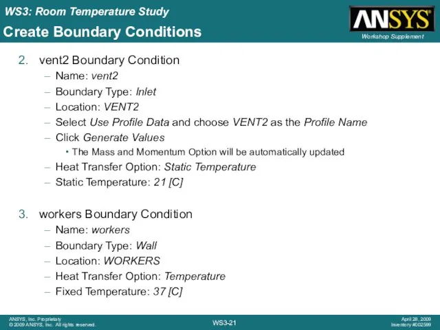
vent2 Boundary Condition
Name: vent2
Boundary Type: Inlet
Location: VENT2
Select Use Profile Data and
vent2 Boundary Condition
Name: vent2
Boundary Type: Inlet
Location: VENT2
Select Use Profile Data and
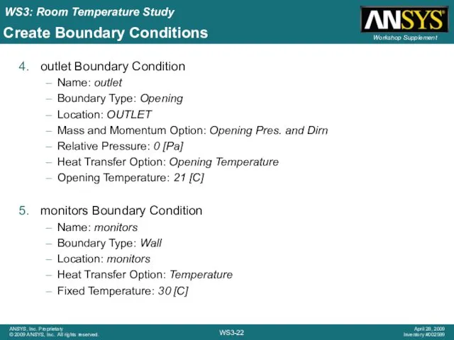
outlet Boundary Condition
Name: outlet
Boundary Type: Opening
Location: OUTLET
Mass and Momentum Option: Opening
outlet Boundary Condition
Name: outlet
Boundary Type: Opening
Location: OUTLET
Mass and Momentum Option: Opening
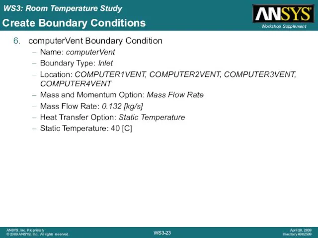
computerVent Boundary Condition
Name: computerVent
Boundary Type: Inlet
Location: COMPUTER1VENT, COMPUTER2VENT, COMPUTER3VENT, COMPUTER4VENT
Mass and
computerVent Boundary Condition
Name: computerVent
Boundary Type: Inlet
Location: COMPUTER1VENT, COMPUTER2VENT, COMPUTER3VENT, COMPUTER4VENT
Mass and
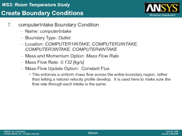
computerIntake Boundary Condition
Name: computerIntake
Boundary Type: Outlet
Location: COMPUTER1INTAKE, COMPUTER2INTAKE, COMPUTER3INTAKE, COMPUTER4INTAKE
Mass and
computerIntake Boundary Condition
Name: computerIntake
Boundary Type: Outlet
Location: COMPUTER1INTAKE, COMPUTER2INTAKE, COMPUTER3INTAKE, COMPUTER4INTAKE
Mass and
Solver Control
Edit Solver Control from the Outline tree
Due to nature of
Solver Control
Edit Solver Control from the Outline tree
Due to nature of
Monitor Point
Edit Output Control from the Outline tree
Switch to the Monitor
Monitor Point
Edit Output Control from the Outline tree
Switch to the Monitor
Monitor Point
In the Expression Value field, type in:
massFlowAve(Temperature)@outlet
Click OK to create
Monitor Point
In the Expression Value field, type in:
massFlowAve(Temperature)@outlet
Click OK to create
Write Solver File
Close CFX-Pre to return to the Project window and
Write Solver File
Close CFX-Pre to return to the Project window and
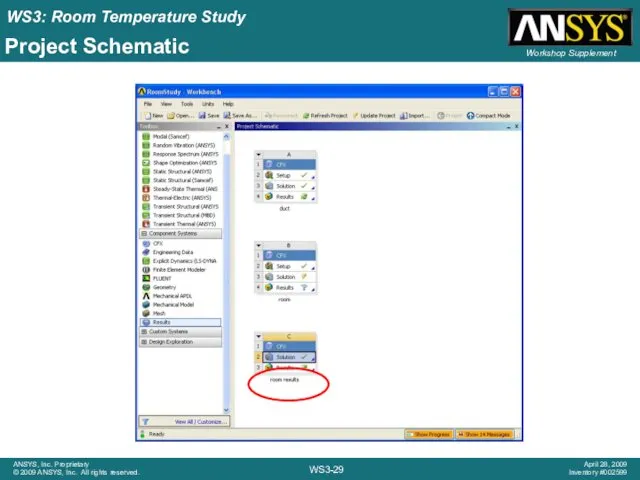
Project Schematic
Project Schematic
CFX Solver Manager
Right-click on Solution in the room results system and
CFX Solver Manager
Right-click on Solution in the room results system and
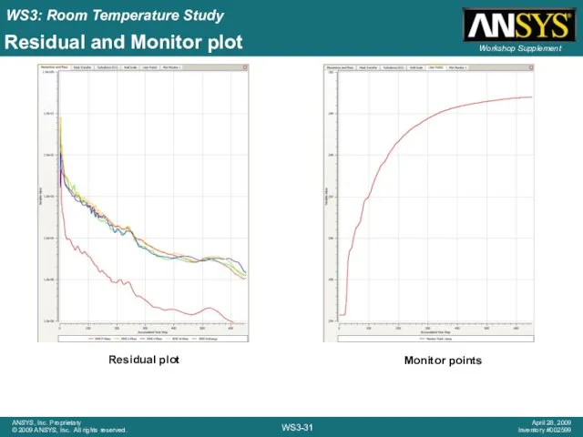
Residual and Monitor plot
Residual plot
Monitor points
Residual and Monitor plot
Residual plot
Monitor points
CFX Solver Manager
Check the Domain Imbalances at the end of the
CFX Solver Manager
Check the Domain Imbalances at the end of the
CFD-Post
Select Location > Plane from the toolbar
In the Details windows on
CFD-Post
Select Location > Plane from the toolbar
In the Details windows on
![CFD-Post ZX Plane at Y = 2 [m] ZX Plane](/_ipx/f_webp&q_80&fit_contain&s_1440x1080/imagesDir/jpg/16074/slide-33.jpg)
CFD-Post
ZX Plane at Y = 2 [m]
ZX Plane at
CFD-Post
ZX Plane at Y = 2 [m]
ZX Plane at

CFD-Post
Click Insert > Vector from the main menu
In the Details windows
CFD-Post
Click Insert > Vector from the main menu
In the Details windows
 ПР4_РОБОТ_Ветвление
 Устройство компьютера
 CoDeSys - общий обзор
 Переменные в Scratch
 Программирование на языке Паскаль (§ 54 - § 61)
 Основи растрової графіки. Використання фото та кліпартів. Растрова анімація
 Как создавать запоминающиеся презентации
 Персональный компьютер
 Внедрение новых технологий Digital Art. Государственная программа Цифровой Казахстан
 Reverse engineering. Обратная разработка и взлом ПО
 Файловая система
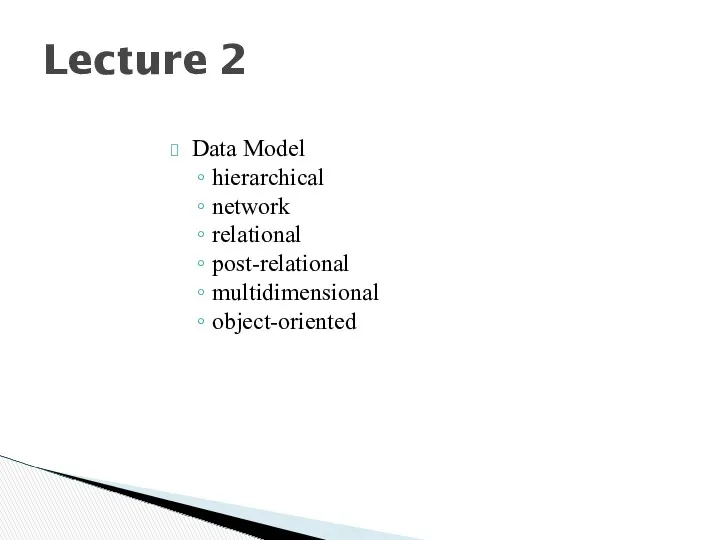 Data Model. Lecture 2
 QOS Requirements and Service Level Agreements. VPN Hose and Pipe Models. Per Flow Sequence Preservation
 switch-case
 Глава 5. Электронные таблицы. Фильтрация данных
 Алгоритм Forel. Выделение устойчивых таксонов
 Мастер-класс. Как прикрепить документы на сайт через Google-диск
 Основы работы с Docker
 Нормативное и правовое обеспечение дополнительного образования детей и молодежи
 Описание структуры документа. XML Schema. (Лекция 3)
 Влияние компьютерных игр на общественное мнение о сексизме, расизме и сексуальных меньшинствах
 Базы данных. Основные понятия и определения
 Текстовые редакторы и текстовые процессоры
 Проект технологического процесса изготовления детали крышка с применением аддитивных технологий
 Электронные таблицы. Ошибки при вводе
 Надежность информации. Основные определения
 Мало известные программы
 Цепочка выполнения программы