- Modeling of nonstationary time series using nonparametric methods

Содержание
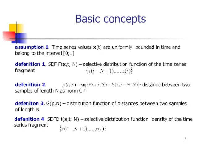
- 2. Basic concepts assumption 1. Time series values x(t) are uniformly bounded in time and belong to
- 3. Let SDFD is a histogram uniformly divided into n class intervals, within which the distribution is
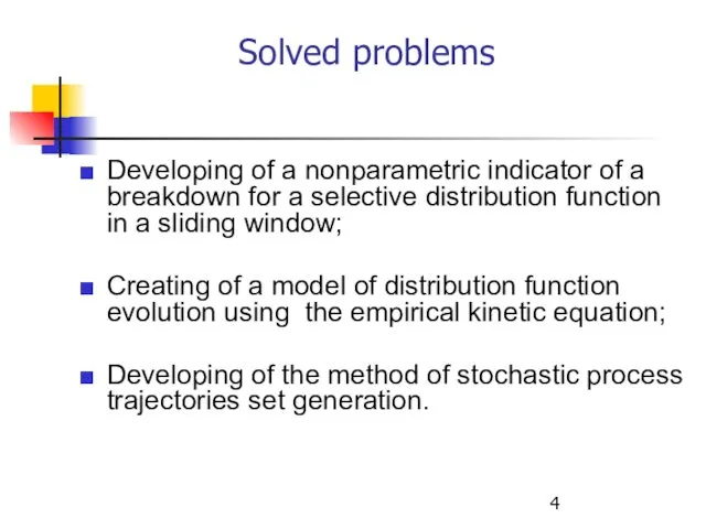
- 4. Solved problems Developing of a nonparametric indicator of a breakdown for a selective distribution function in
- 5. Practical use Earthquake research Medicine Text analysis Telecommunications Stocks market
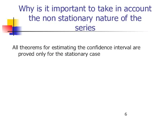
- 6. Why is it important to take in account the non stationary nature of the series All
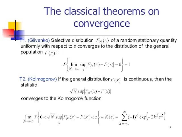
- 7. The classical theorems on convergence Т1. (Glivenko) Selective disribution of a random stationary quantity uniformly with
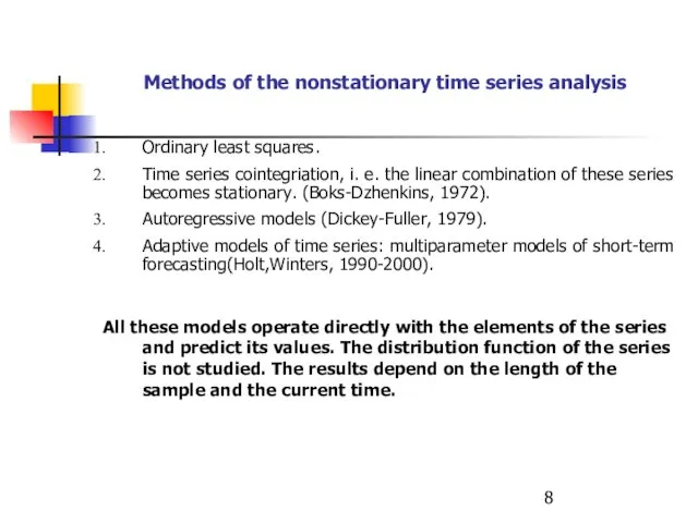
- 8. Methods of the nonstationary time series analysis Ordinary least squares. Time series cointegriation, i. e. the
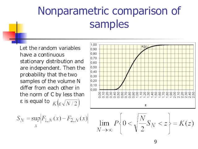
- 9. Nonparametric comparison of samples Let the random variables have a continuous stationary distribution and are independent.
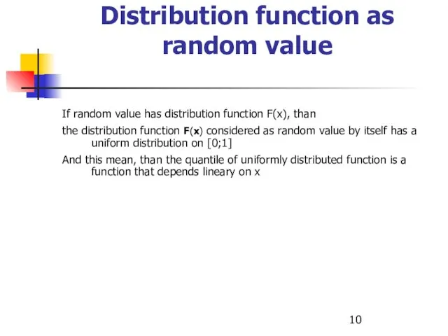
- 10. Distribution function as random value If random value has distribution function F(x), than the distribution function
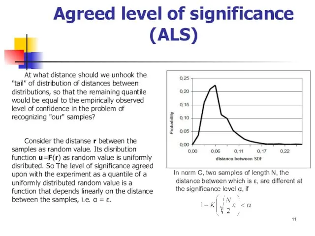
- 11. Agreed level of significance (ALS) At what distance should we unhook the "tail" of distribution of
- 12. The agreed level of significance (stationarity) in the norm of C: the proportion of distances exceeding
- 13. On the left: a series of distances between two samples of length 100 in the norm
- 14. The ALS in the norm of C for stationary disributions does not depend on the type
- 15. If J> 1, the series is nonstationary; if J This approach allows us to introduce not
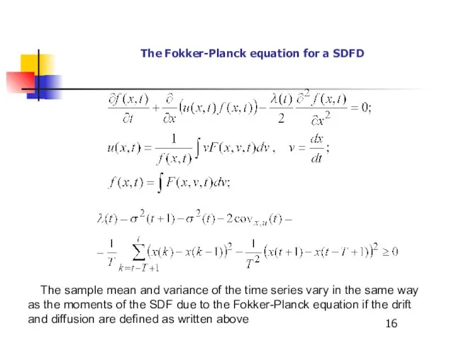
- 16. The Fokker-Planck equation for a SDFD The sample mean and variance of the time series vary
- 17. From the solution of the F-P equation , we know the F (x, t) at all
- 18. Criteria for the correct generation of the ensemble Let we generated s uniformly distributed rows of
- 19. Practical examples Example 1 - earthquake statistics In problems of earthquake prediction the main objects of
- 20. Series ALS depending on the sample length
- 21. Nonstationary index depending on the sample length
- 22. Gutenberg-Richter law for two samples This comparison shows that the nonstationarity of the magnitude distributions can
- 23. Dynamics of the slope angle in the Gutenberg-Richter law The sequence of sample slopes logarithm of
- 24. Autocorrelation analysis of the slope angle Dependence of the autocorrelation selective coefficients of the b(n) series
- 25. The values of the steady-state coefficients of autocorrelation depending on the lag The periodicity of the
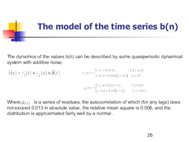
- 26. The model of the time series b(n) The dynamics of the values b(n) can be described
- 27. Nonstationary distributions of magnitudes it was found that the nonstationarity of the distributions magnitude is due
- 28. Earthquake statistics results We analyzed the stationary level of JMA catalog of magnitude and time intervals
- 29. Example 2 - SIR statistics for analysis of 5G networks The reliability of mobile communication is
- 30. From the known distribution function f (x, t), a three-dimensional set of trajectories x (t) is
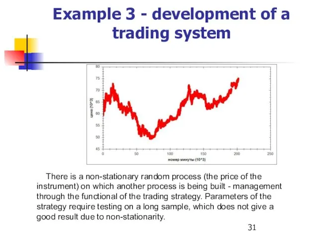
- 31. Example 3 - development of a trading system There is a non-stationary random process (the price
- 32. Problems types Selection of system parameters by historical data Risk-management of a trading System
- 33. Selection of system parameters by historical data A small amount of historical data does not give
- 34. Two types of trajectiories beam generation Generation by historical change of selective distribution. Generation by forecast
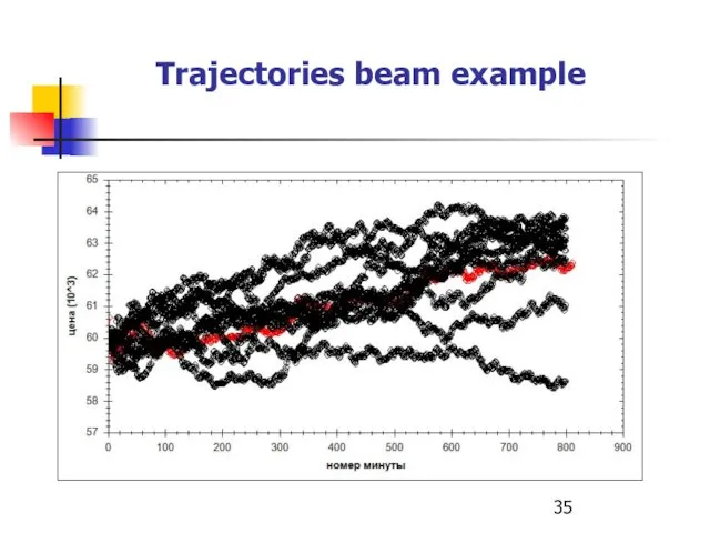
- 35. Trajectories beam example
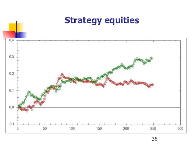
- 36. Strategy equities
- 37. Conclusion Modeling of nonstationary time series has a wide practical application.
- 39. Скачать презентацию
Basic concepts
assumption 1. Time series values x(t) are uniformly bounded
Basic concepts
assumption 1. Time series values x(t) are uniformly bounded
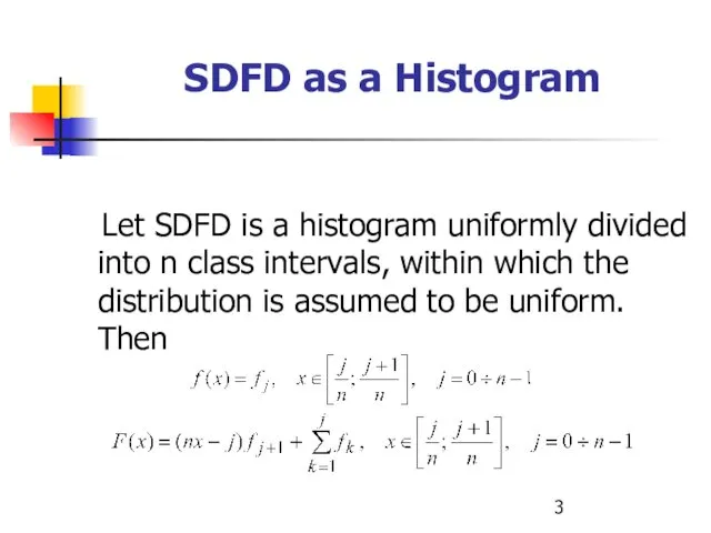
Let SDFD is a histogram uniformly divided into n
Let SDFD is a histogram uniformly divided into n
Solved problems
Developing of a nonparametric indicator of a breakdown for a
Solved problems
Developing of a nonparametric indicator of a breakdown for a
Practical use
Earthquake research
Medicine
Text analysis
Telecommunications
Stocks market
Practical use
Earthquake research
Medicine
Text analysis
Telecommunications
Stocks market
Why is it important to take in account the non stationary
Why is it important to take in account the non stationary
The classical theorems on convergence
Т1. (Glivenko) Selective disribution of a
The classical theorems on convergence
Т1. (Glivenko) Selective disribution of a
Methods of the nonstationary time series analysis
Ordinary least squares.
Time series cointegriation,
Methods of the nonstationary time series analysis
Ordinary least squares.
Time series cointegriation,
Nonparametric comparison of samples
Let the random variables have a continuous
Let the random variables have a continuous
Distribution function as random value
If random value has distribution function F(x),
Distribution function as random value
If random value has distribution function F(x),
Agreed level of significance (ALS)
At what distance should we unhook
Agreed level of significance (ALS)
At what distance should we unhook
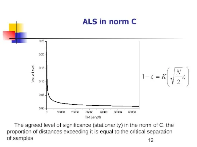
The agreed level of significance (stationarity) in the norm of
The agreed level of significance (stationarity) in the norm of
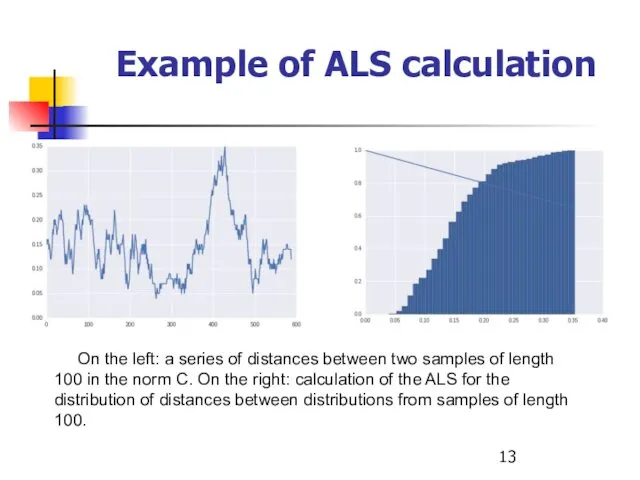
On the left: a series of distances between two samples
On the left: a series of distances between two samples
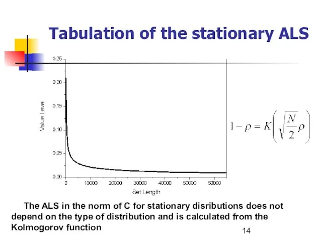
The ALS in the norm of C for stationary disributions
The ALS in the norm of C for stationary disributions
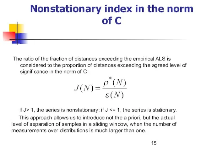
If J> 1, the series is nonstationary; if J <=
If J> 1, the series is nonstationary; if J <=
The Fokker-Planck equation for a SDFD
The sample mean and variance
The sample mean and variance
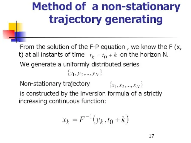
From the solution of the F-P equation , we know
From the solution of the F-P equation , we know
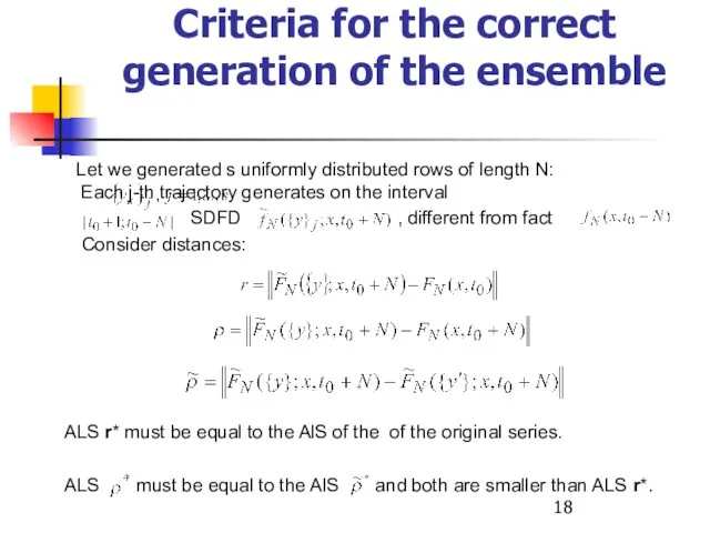
Criteria for the correct generation of the ensemble
Let we generated
Criteria for the correct generation of the ensemble
Let we generated
Practical examples
Example 1 - earthquake statistics
In problems of earthquake prediction the
Practical examples
Example 1 - earthquake statistics
In problems of earthquake prediction the
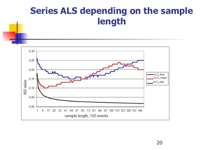
Series ALS depending on the sample length
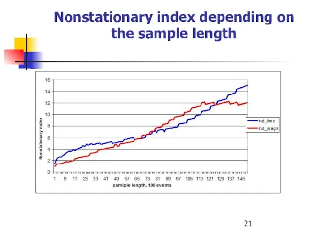
Nonstationary index depending on the sample length
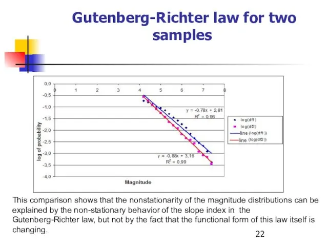
Gutenberg-Richter law for two samples
This comparison shows that the
Gutenberg-Richter law for two samples
This comparison shows that the
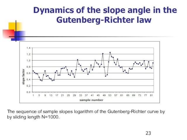
Dynamics of the slope angle in the Gutenberg-Richter law
The
Dynamics of the slope angle in the Gutenberg-Richter law
The
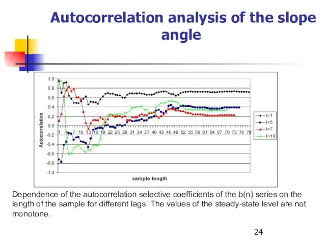
Autocorrelation analysis of the slope angle
Dependence of the
Autocorrelation analysis of the slope angle
Dependence of the
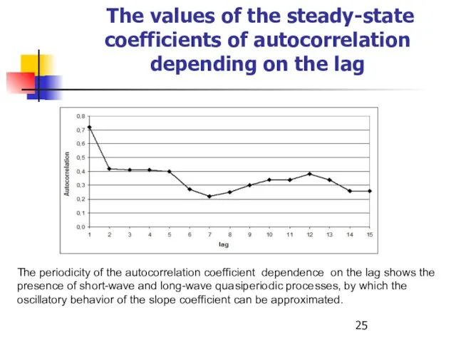
The values of the steady-state coefficients of autocorrelation depending on
The values of the steady-state coefficients of autocorrelation depending on
The model of the time series b(n)
The dynamics of
The model of the time series b(n)
The dynamics of
Nonstationary distributions of magnitudes
it was found that the nonstationarity of
it was found that the nonstationarity of
Earthquake statistics
results
We analyzed the stationary level of JMA catalog of
results
We analyzed the stationary level of JMA catalog of
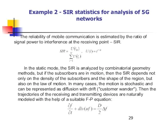
Example 2 - SIR statistics for analysis of 5G networks
Example 2 - SIR statistics for analysis of 5G networks
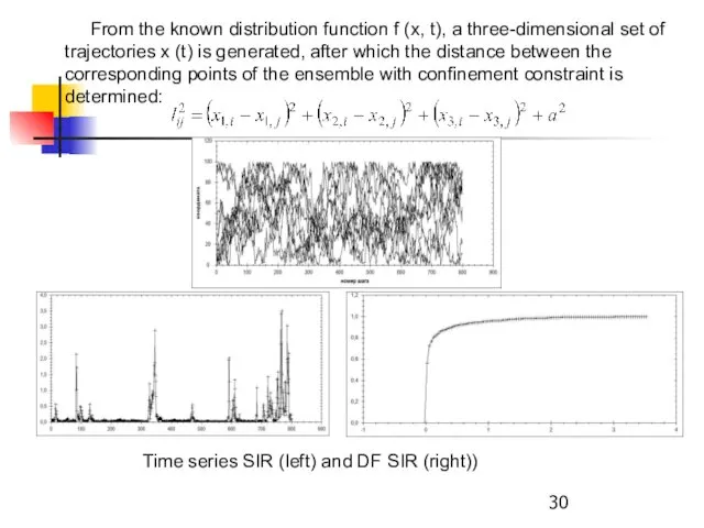
From the known distribution function f (x, t), a three-dimensional
From the known distribution function f (x, t), a three-dimensional
Example 3 - development of a trading system
There is a
There is a
Problems types
Selection of system parameters by historical data
Risk-management of a
Problems types
Selection of system parameters by historical data
Risk-management of a
Selection of system parameters by historical data
A small amount
Selection of system parameters by historical data
A small amount
Two types of trajectiories beam generation
Generation by historical change of
Two types of trajectiories beam generation
Generation by historical change of
Trajectories beam example
Trajectories beam example
Strategy equities
Strategy equities
Conclusion
Modeling of nonstationary time series has a wide practical application.
Conclusion
Modeling of nonstationary time series has a wide practical application.
 Інформаційно-комунікаційні технології професійної діяльності педагога
 Информационные технологии управления
 Введение в специальность. Развитие информационного общества: перспективные направления исследования
 Системы счисления
 The method of software upgrade for tablet PC B902
 WEB GRAPHS/ Modeling the Internet and the Web School of Information and Computer Science
 ГОСТ Р 7.0.100-2018 Одноуровневое библиографическое описание
 Современный образовательный портал MegaCampus
 Цикл с параметром (цикл с заданным числом повторений, цикл-ДЛЯ)
 Створення, відкривання і збереження текстового документа
 Анализ систем управления
 Что делать с неповоротливым JQuery
 Презентация Понятие алгоритма. Исполнители алгоритма. Свойства алгоритма.
 Обработка текстовой и изобразительной информации
 SQL. Манипулирование данными
 Introduction to algorithms and data structures & recursion. Lecture 1. Part I
 Шрифтовый дизайн
 Программа MS Access
 Управление промышленными мехатронными системами
 ВКР: Разработка игрового приложения жанра “Shooter” в среде разработки Unity
 Отечественный опыт развития электронной торговли
 Системы счисления. ОГЭ
 Условные операторы
 Кодирование и обработка звуковой информации
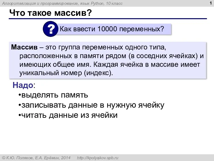 Что такое массив? Алгоритмизация и программирование, язык Python. 10 класс
 Измерение информации. 10 класс
 Установочная лекция по дисциплине Информатика
 Все пути дерева (3 кл)