WEB GRAPHS/ Modeling the Internet and the Web School of Information and Computer Science презентация
- WEB GRAPHS/ Modeling the Internet and the Web School of Information and Computer Science

Содержание
- 2. Internet/Web as Graphs Graph of the physical layer with routers , computers etc as nodes and
- 3. Web Graph http://www.touchgraph.com/TGGoogleBrowser.html
- 4. Web Graph Considerations Edges can be directed or undirected Graph is highly dynamic Nodes and edges
- 5. Why the Web Graph? Example of a large,dynamic and distributed graph Possibly similar to other complex
- 6. Statistics of Interest Size and connectivity of the graph Number of connected components Distribution of pages
- 7. Properties of Web Graphs Connectivity follows a power law distribution The graph is sparse |E| =
- 8. Power Law Size Simple estimates suggest over a billion nodes Distribution of site sizes measured by
- 9. Power Law Connectivity Distribution of number of connections per node follows a power law distribution Study
- 10. Power Law Distribution -Examples http://www.pnas.org/cgi/reprint/99/8/5207.pdf
- 11. Examples of networks with Power Law Distribution Internet at the router and interdomain level Citation network
- 12. Small World Networks It is a ‘small world’ Millions of people. Yet, separated by “six degrees”
- 13. The small world of WWW Empirical study of Web-graph reveals small-world property Average distance (d) in
- 14. Implications for Web Logarithmic scaling of diameter makes future growth of web manageable 10-fold increase of
- 15. Some theoretical considerations Classes of small-world networks Scale-free: Power-law distribution of connectivity over entire range Broad-scale:
- 16. Power Law of PageRank Assess importance of a page relative to a query and rank pages
- 17. PageRank contd Page rank r(v) of page v is the steady state distribution obtained by solving
- 18. Examples Log Plot of PageRank Distribution of Brown Domain (*.brown.edu) G.Pandurangan, P.Raghavan,E.Upfal,”Using PageRank to characterize Webstructure”
- 19. Bow-tie Structure of Web A large scale study (Altavista crawls) reveals interesting properties of web Study
- 20. Bow-tie Components Strongly Connected Component (SCC) Core with small-world property Upstream (IN) Core can’t reach IN
- 21. Component Properties Each component is roughly same size ~50 million nodes Tendrils not connected to SCC
- 22. Empirical Numbers for Bow-tie Maximal minimal (?) diameter 28 for SCC, 500 for entire graph Probability
- 23. Models for the Web Graph Stochastic models that can explain or atleast partially reproduce properties of
- 24. Web Page Growth Empirical studies observe a power law distribution of site sizes Size includes size
- 25. Component One of the Generative Model The first component of this model is that “ sites
- 26. Component Two of the Generative Model There is an overall growth rate α so that the
- 27. Component Two of the Generative Model contd After T steps so that
- 28. Theoretical Considerations Assuming ηt independent, by central limit theorem it is clear that for large values
- 29. Theoretical Considerations contd Log S(T) can also be associated with a binomial distribution counting the number
- 30. Modified Model Can be modified to obey power law distribution Model is modified to include the
- 31. Capturing Power Law Property Inorder to capture Power Law property it is sufficient to consider that
- 32. Lattice Perturbation (LP) Models Some Terms “Organized Networks” (a.k.a Mafia) Each node has same degree k
- 33. Terms (Cont’d) Organized Networks Are ‘cliquish’ (Subgraph that is fully connected) in local neighborhood Probability of
- 34. Semi-organized (SO) Networks Probability for long-range edge is between zero and one Clustered at local level
- 35. Creating SO Networks Step 1: Take a regular network (e.g. lattice) Step 2: Shake it up
- 36. Statistics of SO Networks Average Diameter (d): Average distance between two nodes Average Clique Fraction (c)
- 37. Statistics (Cont’d) Statistics of common networks: Large k = large c? Small c = large d?
- 38. Other Properties For graph to be sparse but connected: n >> k >> log(n) >>1 As
- 39. Effect of ‘Shaking it up’ Small shake (p close to zero) High cliquishness AND short path
- 41. Скачать презентацию
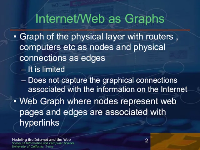
Internet/Web as Graphs
Graph of the physical layer with routers , computers
Internet/Web as Graphs
Graph of the physical layer with routers , computers
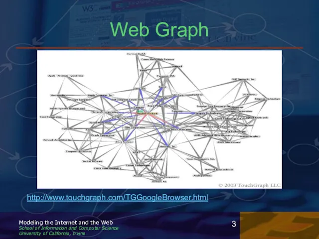
Web Graph
http://www.touchgraph.com/TGGoogleBrowser.html
Web Graph
http://www.touchgraph.com/TGGoogleBrowser.html
Web Graph Considerations
Edges can be directed or undirected
Graph is highly dynamic
Nodes
Web Graph Considerations
Edges can be directed or undirected
Graph is highly dynamic
Nodes
Why the Web Graph?
Example of a large,dynamic and distributed graph
Possibly similar
Why the Web Graph?
Example of a large,dynamic and distributed graph
Possibly similar
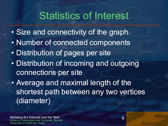
Statistics of Interest
Size and connectivity of the graph
Number of connected components
Distribution
Statistics of Interest
Size and connectivity of the graph
Number of connected components
Distribution
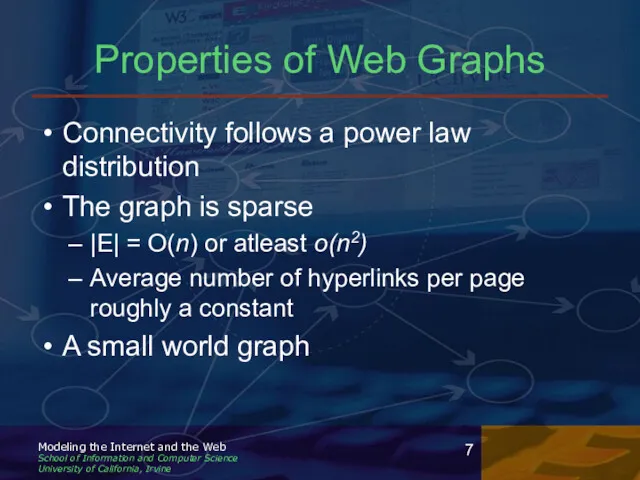
Properties of Web Graphs
Connectivity follows a power law distribution
The graph is
Properties of Web Graphs
Connectivity follows a power law distribution
The graph is
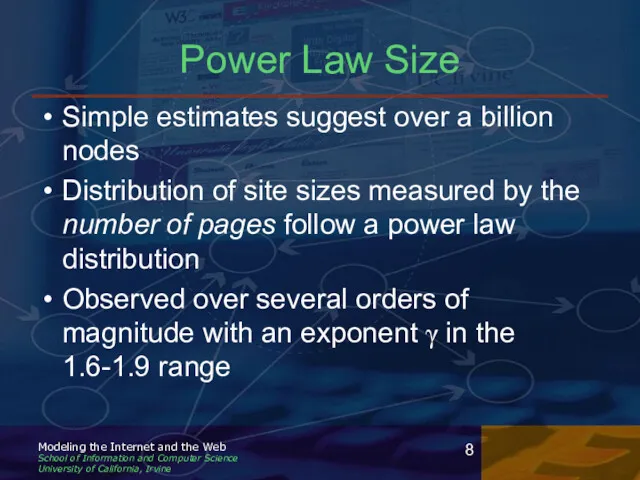
Power Law Size
Simple estimates suggest over a billion nodes
Distribution of site
Power Law Size
Simple estimates suggest over a billion nodes
Distribution of site
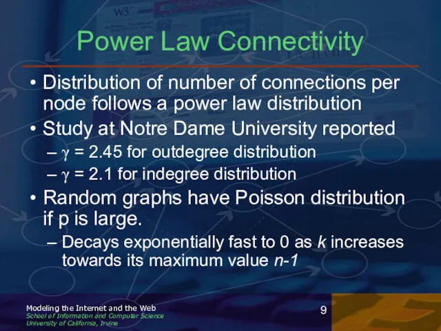
Power Law Connectivity
Distribution of number of connections per node follows a
Power Law Connectivity
Distribution of number of connections per node follows a
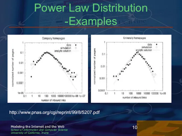
Power Law Distribution -Examples
http://www.pnas.org/cgi/reprint/99/8/5207.pdf
Power Law Distribution -Examples
http://www.pnas.org/cgi/reprint/99/8/5207.pdf
Examples of networks with Power Law Distribution
Internet at the router and
Examples of networks with Power Law Distribution
Internet at the router and
Small World Networks
It is a ‘small world’
Millions of people. Yet, separated
Small World Networks
It is a ‘small world’
Millions of people. Yet, separated
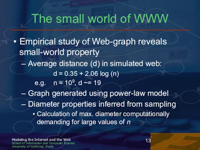
The small world of WWW
Empirical study of Web-graph reveals small-world property
Average
The small world of WWW
Empirical study of Web-graph reveals small-world property
Average
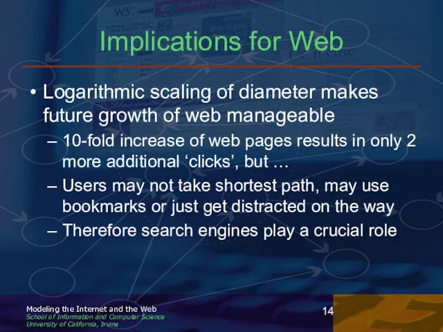
Implications for Web
Logarithmic scaling of diameter makes future growth of web
Implications for Web
Logarithmic scaling of diameter makes future growth of web
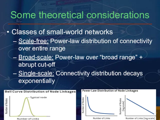
Some theoretical considerations
Classes of small-world networks
Scale-free: Power-law distribution of connectivity over
Some theoretical considerations
Classes of small-world networks
Scale-free: Power-law distribution of connectivity over
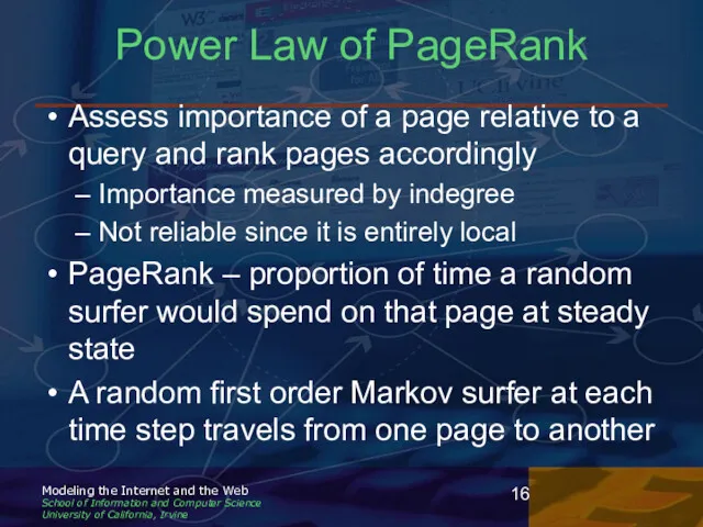
Power Law of PageRank
Assess importance of a page relative to a
Power Law of PageRank
Assess importance of a page relative to a
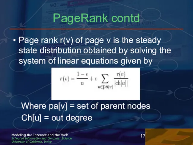
PageRank contd
Page rank r(v) of page v is the steady state
PageRank contd
Page rank r(v) of page v is the steady state
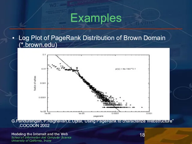
Examples
Log Plot of PageRank Distribution of Brown Domain (*.brown.edu)
G.Pandurangan, P.Raghavan,E.Upfal,”Using PageRank
Examples
Log Plot of PageRank Distribution of Brown Domain (*.brown.edu)
G.Pandurangan, P.Raghavan,E.Upfal,”Using PageRank
Bow-tie Structure of Web
A large scale study (Altavista crawls) reveals interesting
Bow-tie Structure of Web
A large scale study (Altavista crawls) reveals interesting
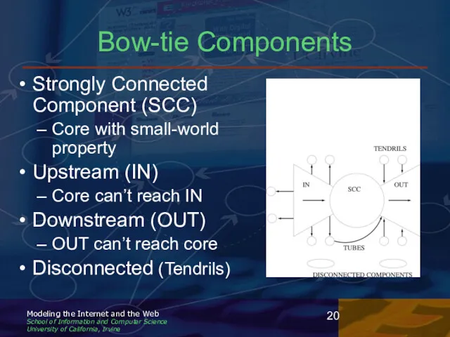
Bow-tie Components
Strongly Connected Component (SCC)
Core with small-world property
Upstream (IN)
Core can’t reach
Bow-tie Components
Strongly Connected Component (SCC)
Core with small-world property
Upstream (IN)
Core can’t reach
Component Properties
Each component is roughly same size
~50 million nodes
Tendrils not connected
Component Properties
Each component is roughly same size
~50 million nodes
Tendrils not connected
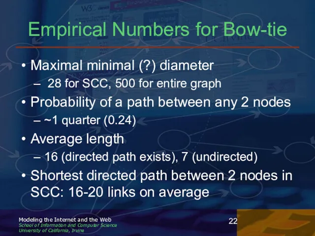
Empirical Numbers for Bow-tie
Maximal minimal (?) diameter
28 for SCC, 500
Empirical Numbers for Bow-tie
Maximal minimal (?) diameter
28 for SCC, 500
Models for the Web Graph
Stochastic models that can explain or atleast
Models for the Web Graph
Stochastic models that can explain or atleast
Web Page Growth
Empirical studies observe a power law distribution of site
Web Page Growth
Empirical studies observe a power law distribution of site
Component One of the Generative Model
The first component of this model
Component One of the Generative Model
The first component of this model
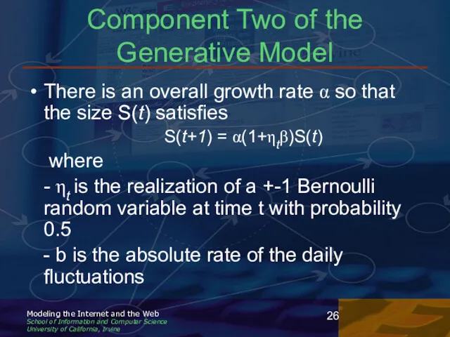
Component Two of the Generative Model
There is an overall growth rate
Component Two of the Generative Model
There is an overall growth rate
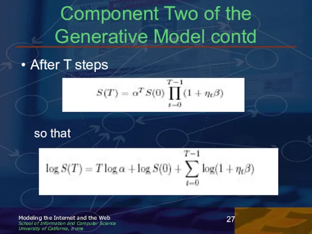
Component Two of the Generative Model contd
After T steps
so that
Component Two of the Generative Model contd
After T steps
so that
Theoretical Considerations
Assuming ηt independent, by central limit theorem it is clear
Theoretical Considerations
Assuming ηt independent, by central limit theorem it is clear
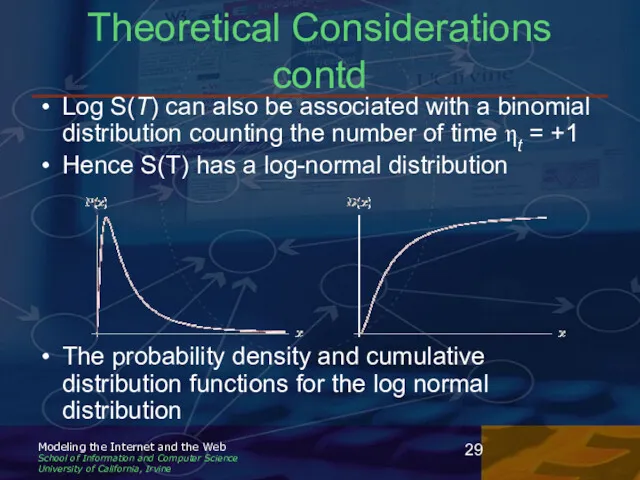
Theoretical Considerations contd
Log S(T) can also be associated with a binomial
Theoretical Considerations contd
Log S(T) can also be associated with a binomial
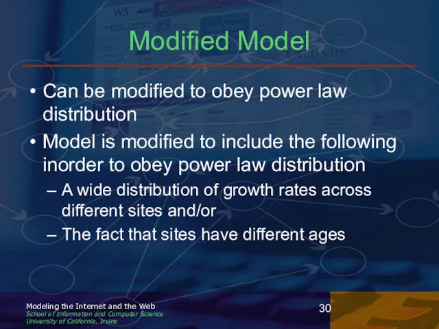
Modified Model
Can be modified to obey power law distribution
Model is modified
Modified Model
Can be modified to obey power law distribution
Model is modified
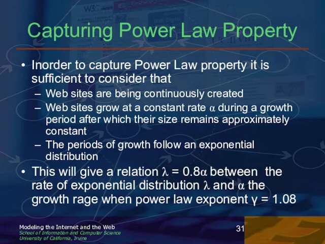
Capturing Power Law Property
Inorder to capture Power Law property it is
Capturing Power Law Property
Inorder to capture Power Law property it is
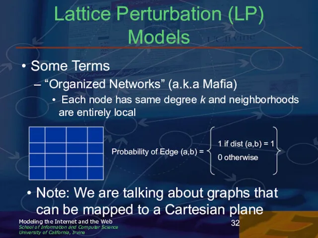
Lattice Perturbation (LP) Models
Some Terms
“Organized Networks” (a.k.a Mafia)
Each node has
Lattice Perturbation (LP) Models
Some Terms
“Organized Networks” (a.k.a Mafia)
Each node has
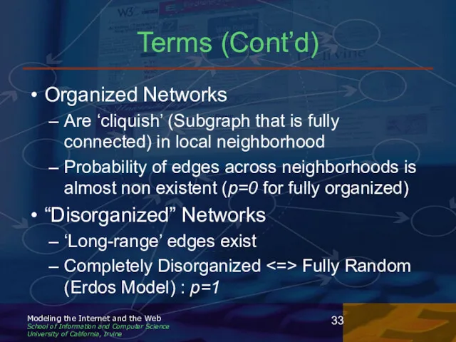
Terms (Cont’d)
Organized Networks
Are ‘cliquish’ (Subgraph that is fully connected) in local
Terms (Cont’d)
Organized Networks
Are ‘cliquish’ (Subgraph that is fully connected) in local
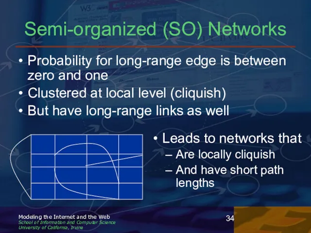
Semi-organized (SO) Networks
Probability for long-range edge is between zero and one
Clustered
Semi-organized (SO) Networks
Probability for long-range edge is between zero and one
Clustered
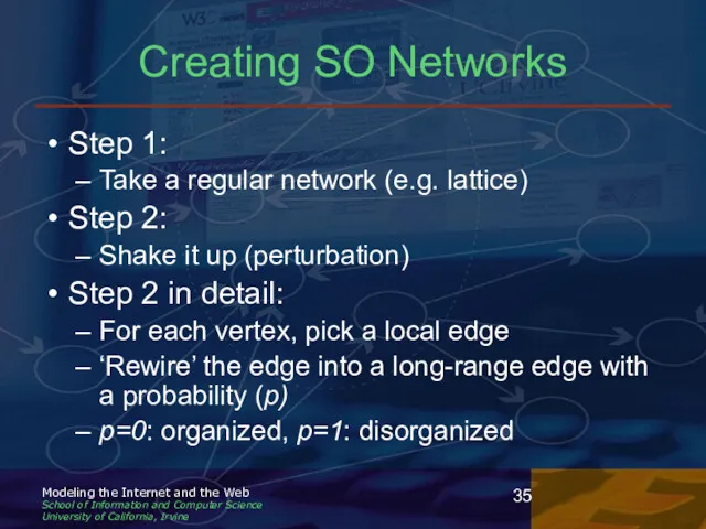
Creating SO Networks
Step 1:
Take a regular network (e.g. lattice)
Step 2:
Shake
Creating SO Networks
Step 1:
Take a regular network (e.g. lattice)
Step 2:
Shake
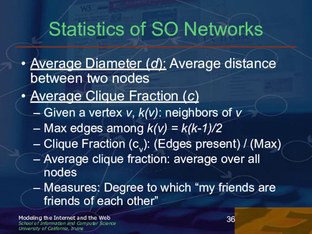
Statistics of SO Networks
Average Diameter (d): Average distance between two
Statistics of SO Networks
Average Diameter (d): Average distance between two
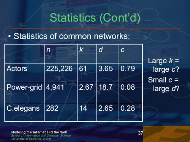
Statistics (Cont’d)
Statistics of common networks:
Large k = large c?
Small
Statistics (Cont’d)
Statistics of common networks:
Large k = large c?
Small
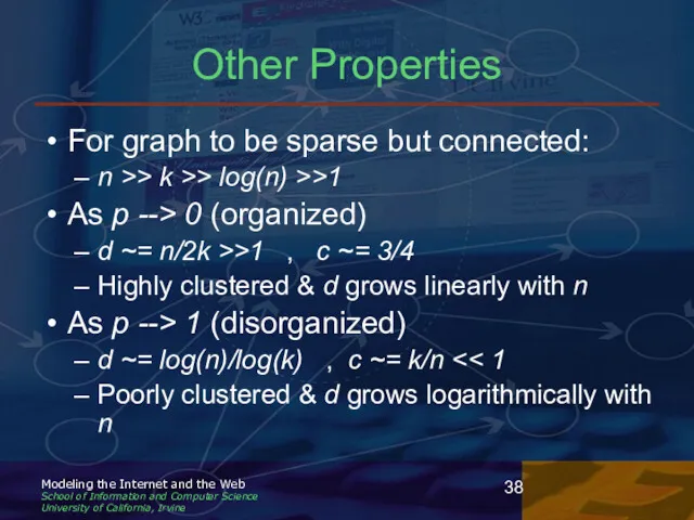
Other Properties
For graph to be sparse but connected:
n >> k >>
Other Properties
For graph to be sparse but connected:
n >> k >>
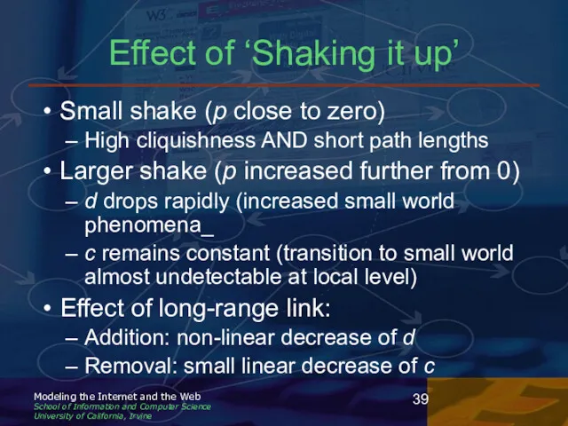
Effect of ‘Shaking it up’
Small shake (p close to zero)
High cliquishness
Effect of ‘Shaking it up’
Small shake (p close to zero)
High cliquishness
 Информационная безопасность
 GSIS Инструкция пользователя (Для сервисного центра)
 Образовательный видео сервис
 Microsoft Word кестелер, суреттер және су белгілерін енгізу
 Прерывания в системах DOS и BIOS. (Лекция 13)
 Powercode academy
 Об’єкт event. Обробка подій
 Внеклассное мероприятие по информатике. Анаграммы
 Хранение однотипных данных. Массивы
 Корпоративные системы электронного документооборота. Обзор ECM решений
 Разработка Телеграм-бота для предприятия ООО “Элегия”
 Каналы передачи информации
 Интернет-магазин подарков ручной работы
 Исследование возможностей применения BIM-технологии в компьютерном дизайне (на примере интерьера загородного дома)
 Как варить подкасты
 Adobe Illustrator программасының интерфейсі
 Основные алгоритмические конструкции
 Распространенные форматы графических файлов, их преимущества, недостатки и области применения
 Оформление списка литературы. Библиографические БД
 Назначение блоков персонального компьютера (ПК)
 Хранение информации. Память человека и память человечества. Оперативная и долговременная память. Файлы и папки. (5 класс)
 Microsoft excel Терезесіне шолу
 World Wide Web – Всемирная Паутина
 Знания. Конкурс Интеллектуальная собственность глазами молодежи
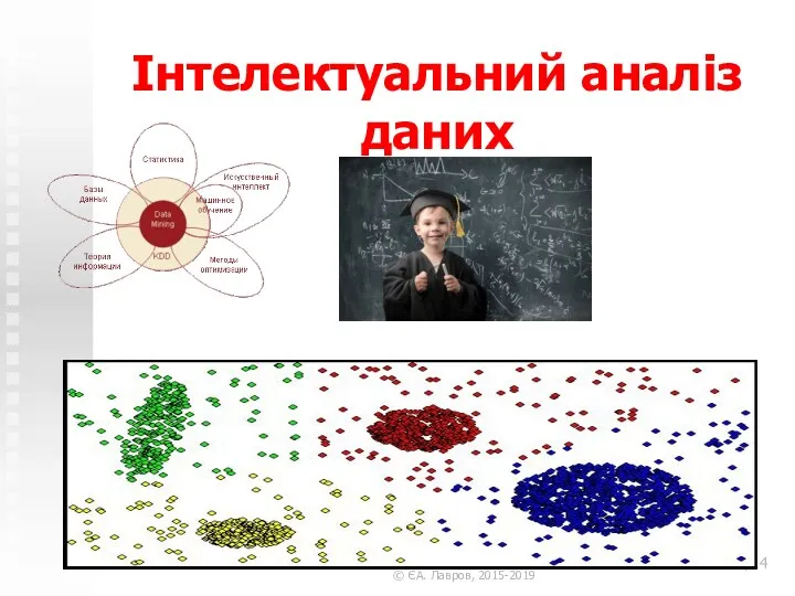 Інтелектуальний аналіз даних
 Операционные системы для мобильных устройств
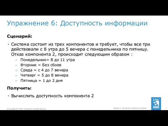 Упражнение 6: Доступность информации
 Обработка текстовой информации. Текстовый редактор