- Programming in the Integrated Environments. Programming in the Scilab system

Содержание
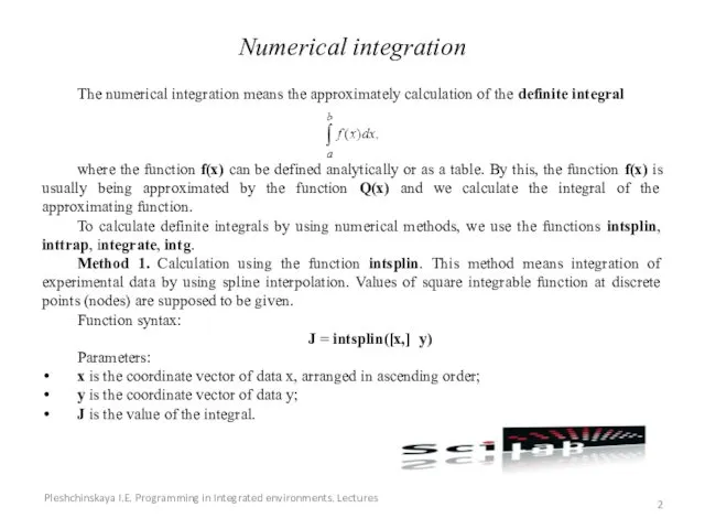
- 2. Numerical integration The numerical integration means the approximately calculation of the definite integral where the function
- 3. Example. Calculate the integral of a function given by the table --> x = 1:.4:5; -->
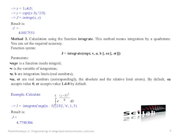
- 4. --> x = 1:.4:5; --> y = exp((x-3).^2/8) --> J = inttrap(x, y) Result is: J
- 5. You can use another method also: create the file-function a.sci function g = a(x) g =
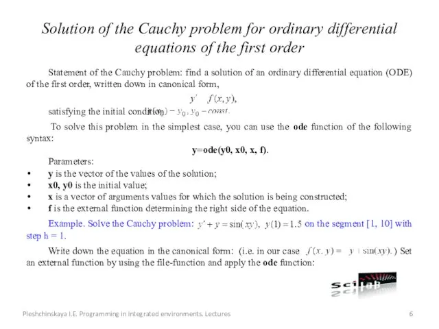
- 6. Solution of the Cauchy problem for ordinary differential equations of the first order Statement of the
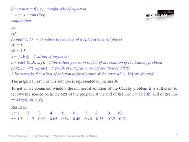
- 7. function w = f(x, y) // right side of equation w = -y + sin(x*y); endfunction
- 8. Figure 30. Graphical solution of the Cauchy problem By using the ode function, it is possible
- 9. Pleshchinskaya I.E. Programming in Integrated environments. Lectures The initial condition in this case has the same
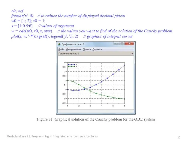
- 10. clc, scf format('v', 5) // to reduce the number of displayed decimal places w0 = [1;
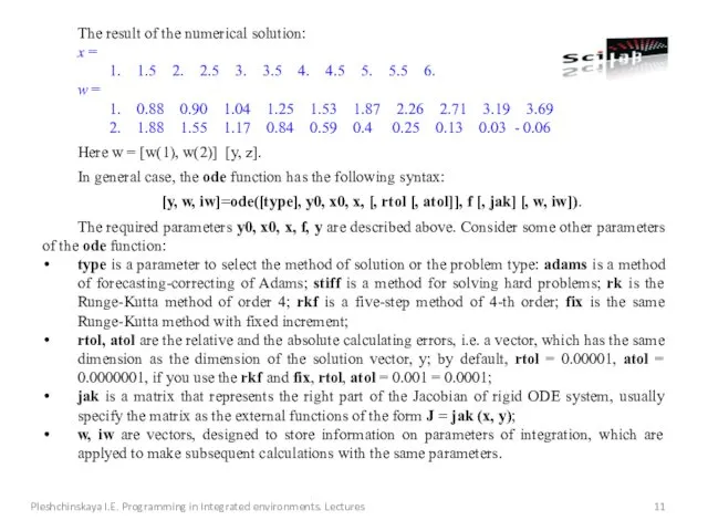
- 11. The result of the numerical solution: x = 1. 1.5 2. 2.5 3. 3.5 4. 4.5
- 12. Linear programming problems Linear programming problems are the problems of the multidimensional optimization, in which the
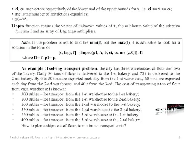
- 13. ci, cs are vectors respectively of the lower and of the upper bounds for x, i.e.
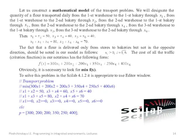
- 14. Pleshchinskaya I.E. Programming in Integrated environments. Lectures Let us construct a mathematical model of the transport
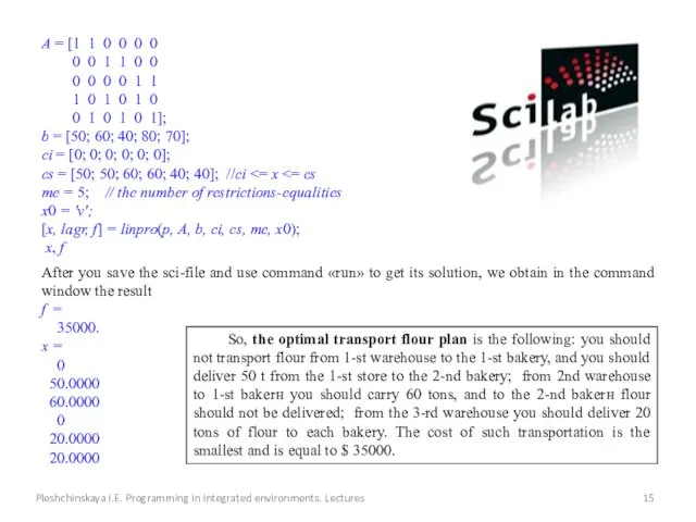
- 15. A = [1 1 0 0 0 0 0 0 1 1 0 0 0 0
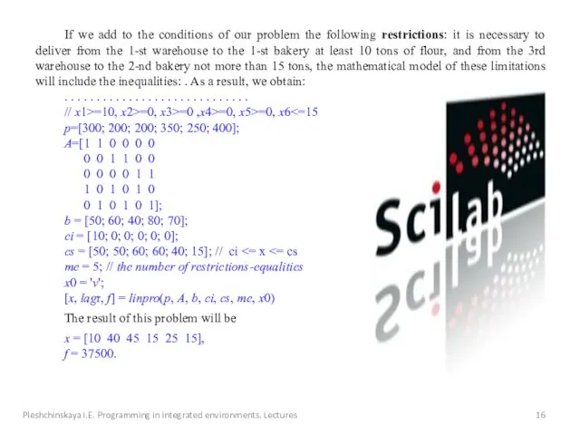
- 16. If we add to the conditions of our problem the following restrictions: it is necessary to
- 17. An example of solving the production planning problem: furniture workshop produces two types of chairs. One
- 18. The result x = 60 80 f1= 1440 So, if we produce 60 chairs of the
- 19. Let us solve the previous problem in Scilab 5.4.0. We input in the Editor window the
- 21. Скачать презентацию
Numerical integration
The numerical integration means the approximately calculation of the
Numerical integration
The numerical integration means the approximately calculation of the

Example. Calculate the integral of a function given by the table
-->
Example. Calculate the integral of a function given by the table
-->
--> x = 1:.4:5;
--> y = exp((x-3).^2/8)
--> J = inttrap(x, y)
Result
--> x = 1:.4:5;
--> y = exp((x-3).^2/8)
--> J = inttrap(x, y)
Result
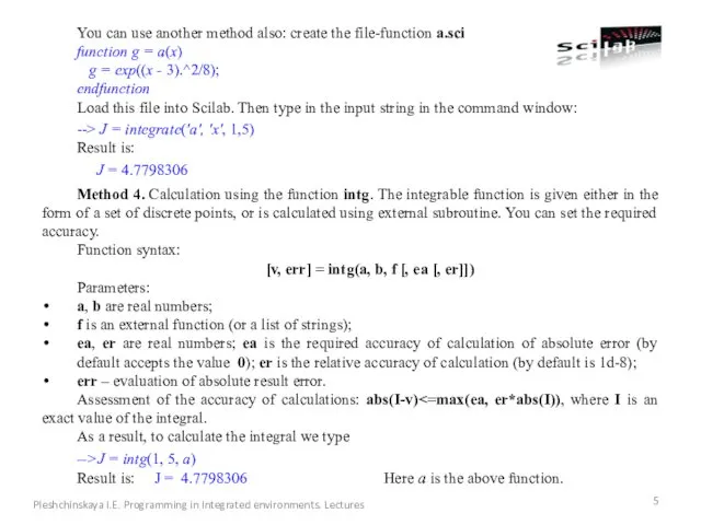
You can use another method also: create the file-function a.sci
function
You can use another method also: create the file-function a.sci
function
Solution of the Cauchy problem for ordinary differential equations of the
Solution of the Cauchy problem for ordinary differential equations of the
function w = f(x, y) // right side of equation
w
function w = f(x, y) // right side of equation
w
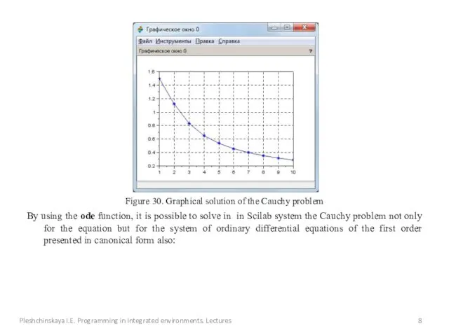
Figure 30. Graphical solution of the Cauchy problem
By using the ode
Figure 30. Graphical solution of the Cauchy problem
By using the ode

Pleshchinskaya I.E. Programming in Integrated environments. Lectures
The initial condition in this
Pleshchinskaya I.E. Programming in Integrated environments. Lectures
The initial condition in this
clc, scf
format('v', 5) // to reduce the number of displayed decimal
clc, scf
format('v', 5) // to reduce the number of displayed decimal
The result of the numerical solution:
x =
1. 1.5 2. 2.5
The result of the numerical solution:
x =
1. 1.5 2. 2.5

Linear programming problems
Linear programming problems are the problems of the multidimensional
Linear programming problems
Linear programming problems are the problems of the multidimensional
ci, cs are vectors respectively of the lower and of the
ci, cs are vectors respectively of the lower and of the
Pleshchinskaya I.E. Programming in Integrated environments. Lectures
Let us construct a mathematical
Pleshchinskaya I.E. Programming in Integrated environments. Lectures
Let us construct a mathematical
A = [1 1 0 0 0 0
0 0 1
A = [1 1 0 0 0 0
0 0 1
If we add to the conditions of our problem the following
If we add to the conditions of our problem the following
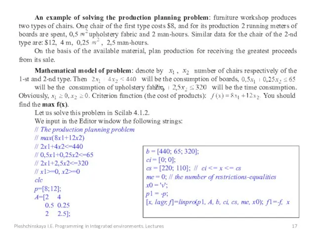
An example of solving the production planning problem: furniture workshop produces
An example of solving the production planning problem: furniture workshop produces
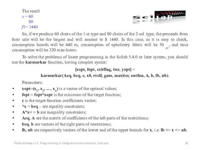
The result
x = 60
80
f1= 1440
So, if we produce 60 chairs
The result
x = 60
80
f1= 1440
So, if we produce 60 chairs

Let us solve the previous problem in Scilab 5.4.0.
We input in
Let us solve the previous problem in Scilab 5.4.0.
We input in
 Миниатюра аватара
 Жизненный цикл информационных систем
 Ұғымдардың атауы: программа, программалаудың деңгейлері және дәрежелері (бағыттары), программаларды өңдеу және аспаптары
 создание тура в программе Мастер-Тур
 Вычислительные системы, сети и телекоммуникации. Введение
 Разработка Web-сайта 2019 год – год театра
 Кейсы окупаемости Focus для ТЦ
 Решение задач в Excel
 Как устроен интернет
 Комп’ютерна верстка
 урок информатики по учебнику Плаксина М.А. тема Как управлять компьютером с помощью клавиатуры
 Разработка ТЗ
 GitHub - найбільший веб-сервіс для хостингу IT-проектів і їх спільної розробки
 Презентация к интегрированному уроку Пословицы и поговорки
 Язык программирования Python. Процедуры и функции в языке Python
 Анализ еженедельного вечернего выпуска новостей телеканала НТВ
 Архитектура компьютера открытый урок
 Информатика лидері
 Компьютерные презентации. Разработка и создание презентации
 IV поколение ЭВМ
 Безпека інформаційних технологій. Інформація та інформаційні відносини. Урок 1. Інформатика. 10(11) клас
 Влияние социальных сетей на личность подростка
 Анализ бизнес-процессов средствами BPwin
 3D принтеры
 Установка Microsoft Office
 Физминутка
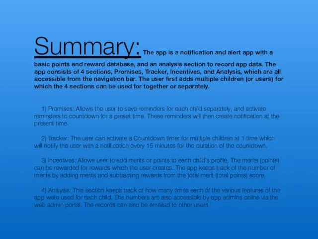 The app is a notification and alert app with a basic points and reward database, and an analysis section to record app data
 Кодирование и декодирование информации