- Simulia - solutions for turbomachinery

Содержание
- 2. Agenda Turbomachinery update – Jack Cofer Vision for next three years Mechanisms for prioritizing product enhancements
- 3. Agenda (Siemens) Turbomachinery update – Jack Cofer Vision for next three years Future roadmaps Improvements in
- 4. SIMULIA Turbomachinery Vision – Next 3 Years Major components of the Turbo Industry vision: Work closely
- 5. Mechanisms for Prioritizing Requests for Enhancements Customers submit RFEs through their local offices Offices review them
- 6. Future Simulation Roadmaps Simulation Roadmaps drive product development to increase our competitiveness per industry Owned and
- 7. Rotordynamics Plug-in to automatically generate Campbell diagrams – see Abaqus Answer #4721 Plug-in to enable direct
- 8. UVA Rotating Machinery and Controls Laboratory (ROMAC) Industrial Program In June 2010, SIMULIA joined the University
- 9. Joint Rotordynamics Work with ROMAC Dr. Youngwon Hahn is currently working with two Ph.D. students at
- 10. Major RFE Status (Siemens) Mapping issues Displaying contour plots of all loads/boundaries/fields (including film conditions) in
- 11. Abaqus 6.11 Preview SIMULIA Technical Marketing
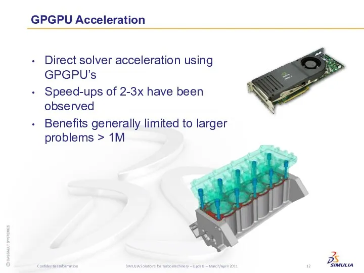
- 12. GPGPU Acceleration Direct solver acceleration using GPGPU’s Speed-ups of 2-3x have been observed Benefits generally limited
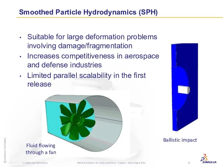
- 13. Suitable for large deformation problems involving damage/fragmentation Increases competitiveness in aerospace and defense industries Limited parallel
- 14. Contact pressure error indicators increase confidence in results quality Edge-surface contact expands the class of problems
- 15. Conveyer Belt Specialized technique for simulating continuous processes Limited to periodic geometries Unique in the industry
- 16. Parallel Frequency Response Solver Targeted towards automotive NV market Supports SMP w/ up to 24 cores
- 17. Multiphysics New solution procedures for: Thermal-electrical-structural (ETS) Low-frequency electromagnetics (EM) Sequential thermal-stress following EM Applications span
- 18. CATIA V5 Bidirectional Associative Interface CATIA parameters can be modified from Abaqus/CAE Model updated automatically Support
- 19. Substructures Continuation of 6.10-EF project Support for: Substructure load cases Substructure load Improved display Substructure statistics
- 20. Reduce picking needed to create mid-surface Improved robustness Offset operation performance Feature regeneration Enhanced heuristics for
- 21. Tet Meshing Minimum element size specification Tetrahedral element size growth control for interior volume Improved quality
- 22. New mesh edit functions Merge/subdivide elements Grow/collapse short element edges Bottom-up meshing Now available for orphan
- 23. Mapping Capability Interface for: Importing spatially varying point cloud field data Applying data sets as loads,
- 24. Capabilities for realistic modeling of fasteners Create Template model Separate from actual analysis model. Contains surfaces,
- 25. Analysis Coverage Interface for Anisotropic Hyperelasticity Highly anisotropic and nonlinear elastic material behavior Model soft biological
- 26. Abaqus Topology Optimization Module (ATOM) Topology optimization Modify stiffness Good for evolving optimum shape Shape optimization
- 27. Contour plots on beam sections Available for Box, Rectangle, Circle, Pipe, I and L sections New
- 28. Section force/moment history output Section force/moment display on multiple view cuts Multiple free bodies on a
- 29. Isight 5.5 Preview SIMULIA Technical Marketing
- 30. Intuitive graphical interface Integrate applications and automate simulation processes using components Full suite of powerful exploration
- 31. Isight 5.5 Enhancements Model & Simulation Integration Dymola component Model comparison tool Optimization MISQP Custom exploration
- 32. Isight 5.5 Enhancements: Model & Simulation Integration Dymola Component allows users to modify a Dymola input
- 33. Python/Jython, Java script mode offers complete flexibility to impose any desired logic on the optimization process
- 34. Isight 5.5 Enhancement: Mixed-Integer Sequential Quadratic Programming Algorithm (MISQP) Excellent benchmark results: #function calls for each
- 35. 2011 SIMULIA Customer Conference Advanced Seminars - May 16; Conference - May 17-19, 2011 Barcelona, Spain
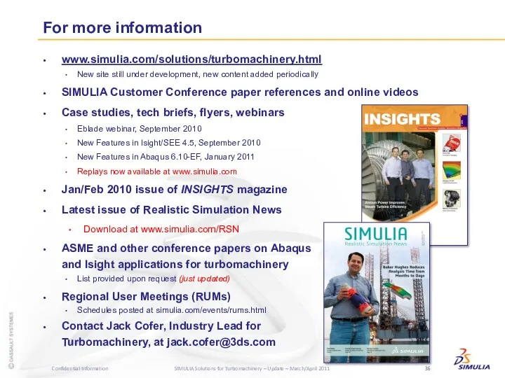
- 36. www.simulia.com/solutions/turbomachinery.html New site still under development, new content added periodically SIMULIA Customer Conference paper references and
- 37. Turbomachinery Applications using Abaqus Youngwon Hahn Ver. OCT 2010
- 38. Who Is Dr. Youngwon Hahn?
- 39. Overview Rotordynamics Gyroscopic Effect Bearing Modeling Frequency Extraction and Frequency Response Campbell Diagram Plug-in Other Plug-in
- 40. Rotordynamics
- 41. Rotordynamics Abaqus provides two approaches for gyroscopic effect. Eulerian approach This technique was required by a
- 42. Rotordynamics Lagrangian approach General approach. User can apply body force as the function of the spin
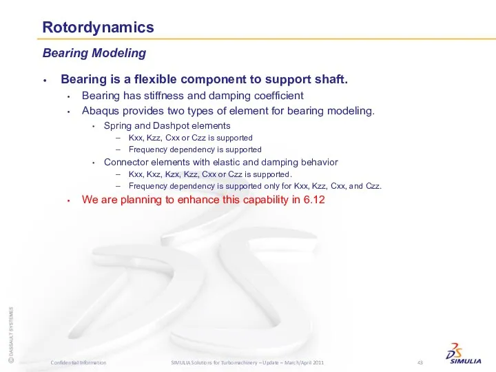
- 43. Rotordynamics Bearing is a flexible component to support shaft. Bearing has stiffness and damping coefficient Abaqus
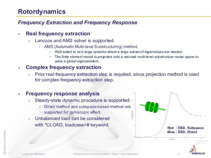
- 44. Rotordynamics Real frequency extraction Lanczos and AMS solver is supported. AMS (Automatic Multi-level Substructuring) method Well-suited
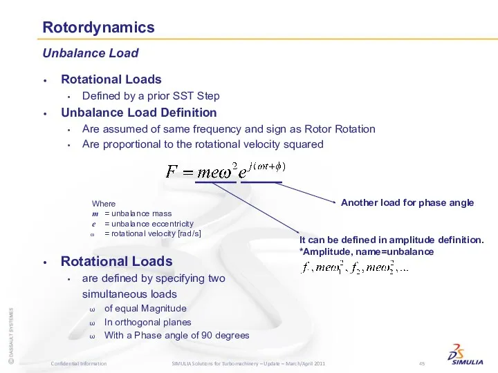
- 45. Rotordynamics Rotational Loads Defined by a prior SST Step Unbalance Load Definition Are assumed of same
- 46. Introduction Complex plane The time variation of an excitation or output quantity during a cycle of
- 47. Rotordynamics Complex axes to physical axes Example: Unit force due to an imbalance for a z-axis
- 48. Rotordynamics Use right-hand rule To define 1-axis in the direction of real force at time=0 and
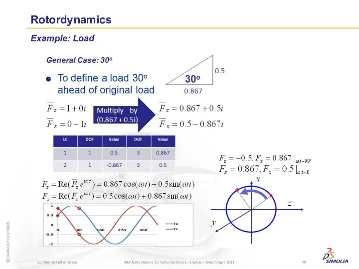
- 49. Rotordynamics Example: Load
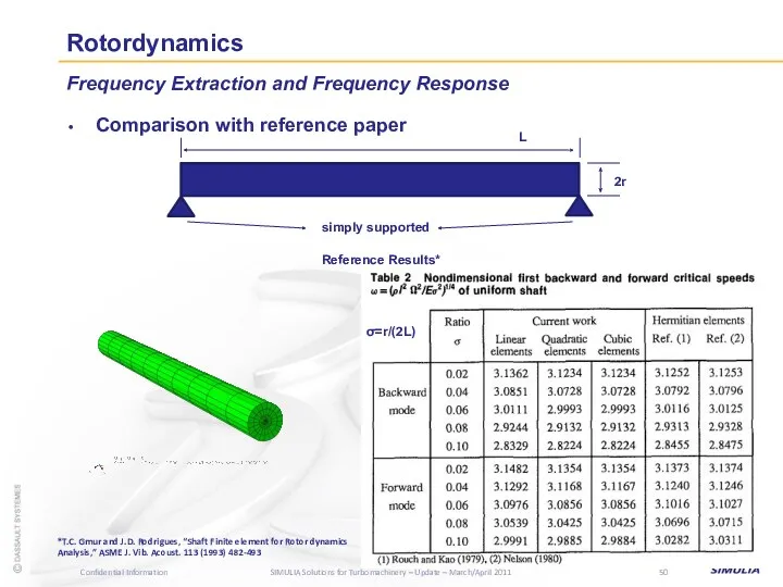
- 50. Rotordynamics Comparison with reference paper Frequency Extraction and Frequency Response Reference Results* *T.C. Gmur and J.D.
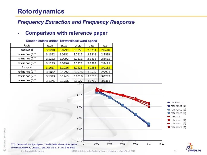
- 51. Rotordynamics Comparison with reference paper Frequency Extraction and Frequency Response *T.C. Gmur and J.D. Rodrigues, “Shaft
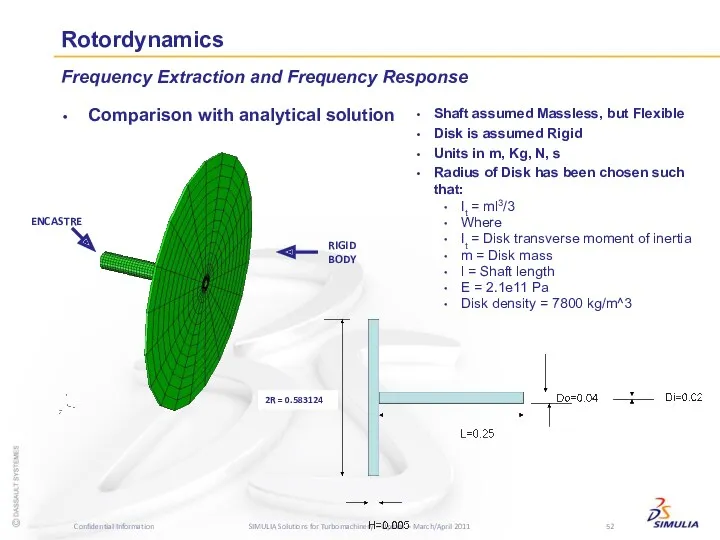
- 52. Rotordynamics Comparison with analytical solution Frequency Extraction and Frequency Response Shaft assumed Massless, but Flexible Disk
- 53. Rotordynamics Comparison with analytical solution Frequency Extraction and Frequency Response *J.P. Den Hartog, “Mechanical Vibrations,” Dover
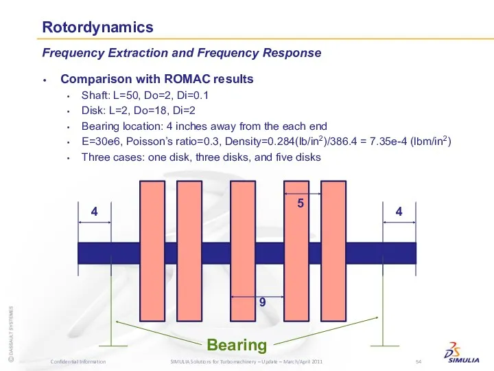
- 54. Rotordynamics Comparison with ROMAC results Shaft: L=50, Do=2, Di=0.1 Disk: L=2, Do=18, Di=2 Bearing location: 4
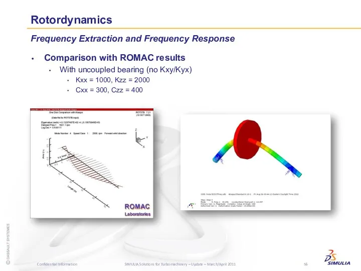
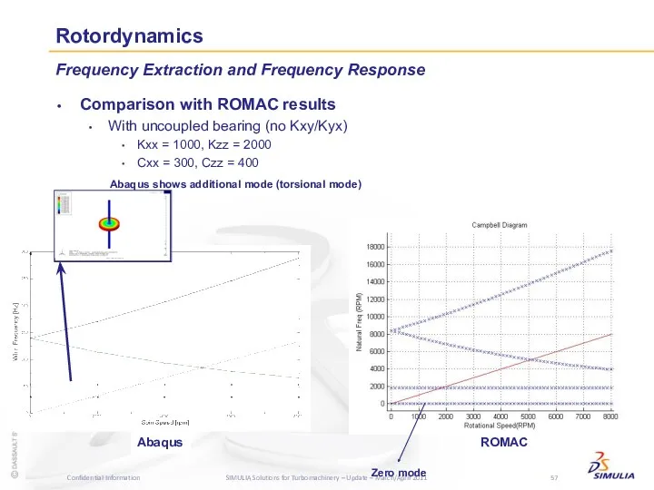
- 55. Rotordynamics Comparison with ROMAC results With uncoupled bearing (no Kxy/Kyx) Kxx = 1000, Kzz = 2000
- 56. Rotordynamics Comparison with ROMAC results With uncoupled bearing (no Kxy/Kyx) Kxx = 1000, Kzz = 2000
- 57. Rotordynamics Comparison with ROMAC results With uncoupled bearing (no Kxy/Kyx) Kxx = 1000, Kzz = 2000
- 58. Rotordynamics Load Definition (unbalance load) 1 oz-in at 0,90, and180 degrees (X-axis is 0 degree) Frequency
- 59. Simple Rotor (Three Disks) Frequency Extraction and Frequency Response
- 60. Rotordynamics Newly developed A/Viewer Plug-in for rotordynamic application Campbell Diagram Plug-in (ANSWER 4721)
- 61. Rotordynamics Newly developed A/Viewer Plug-in for rotordynamic application Campbell Diagram Plug-in Reference curve
- 62. Rotordynamics Plug-in to import bearing property from ROMAC Bearing Code (THBRG, THPAD, and MAXBRG) Other Plug-in
- 63. Rotordynamics Plug-in to import bearing property from ROMAC Bearing Code (THBRG, THPAD, and MAXBRG) Calculate Coefficients
- 64. Rotordynamics Plug-in to import bearing property from ROMAC Bearing Code (THBRG, THPAD, and MAXBRG) Manual Input
- 65. Rotordynamics Plug-in to import bearing property from ROMAC Bearing Code (THBRG, THPAD, and MAXBRG) Read from
- 66. Rotordynamics Abaqus provides substructuring capability (superelement). Gyroscopic effect is handled as a damping matrix. Abaqus supports
- 67. Rotordynamics Example: Rotor-bearing system with support structure. Modal analysis considering spin speed (261 rad/s) Bearing with
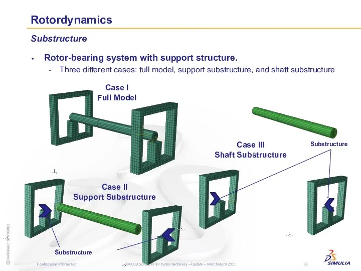
- 68. Rotordynamics Rotor-bearing system with support structure. Three different cases: full model, support substructure, and shaft substructure
- 69. Rotordynamics Rotor-bearing system with support structure. Three different cases: full model, support substructure, and shaft substructure
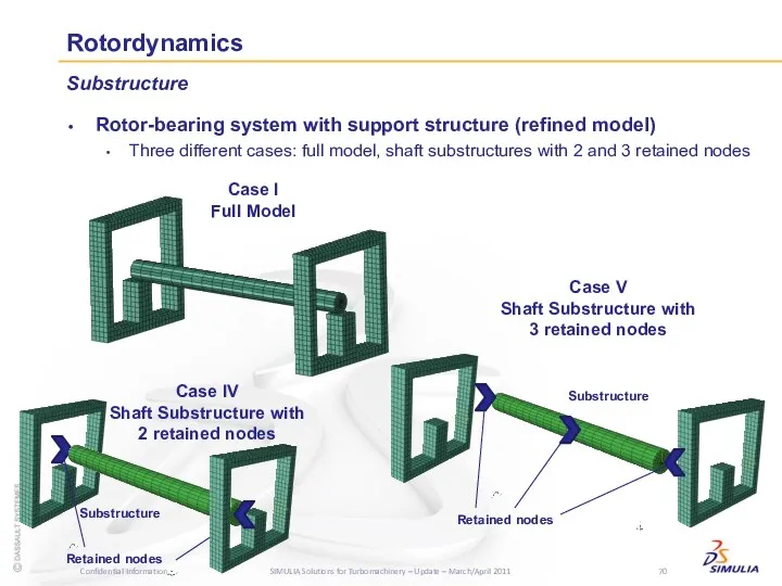
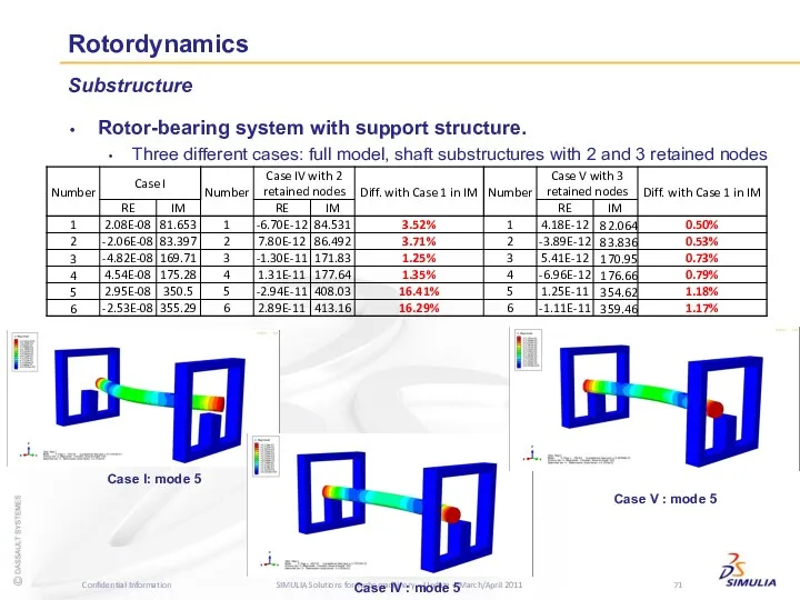
- 70. Rotordynamics Rotor-bearing system with support structure (refined model) Three different cases: full model, shaft substructures with
- 71. Rotordynamics Rotor-bearing system with support structure. Three different cases: full model, shaft substructures with 2 and
- 72. Coupled Structural-Acoustic Analysis
- 73. Coupled Structural-Acoustic Analysis Lanczos and AMS solvers support coupled structural-acoustic analysis. We have two kinds of
- 74. Coupled Structural-Acoustic Analysis Coupled Structural Acoustic Model Steel thickness: 1.219 mm length: 1010 mm mean radius:
- 75. Coupled Structural-Acoustic Analysis Coupled Structural Acoustic Model Result Frequency range: 80-480 Hz *S. Boily and F.
- 76. Blade Analysis
- 77. Blade Analysis Blade Geometry from Eblade (see appendix for more details) Modeling in A/CAE
- 78. Blade Analysis Import Eblade data to A/CAE: Plug-in Number of section Number of points coordinates The
- 79. Blade Analysis Create geometry by Loft Repeat…
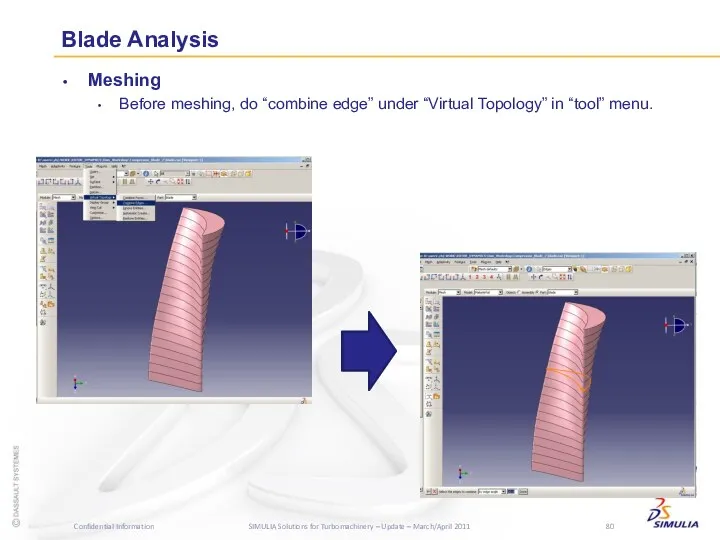
- 80. Blade Analysis Meshing Before meshing, do “combine edge” under “Virtual Topology” in “tool” menu.
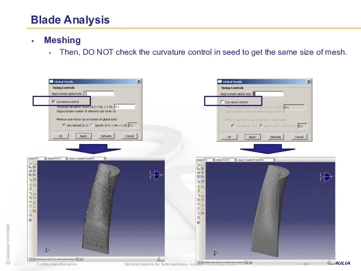
- 81. Blade Analysis Meshing Then, DO NOT check the curvature control in seed to get the same
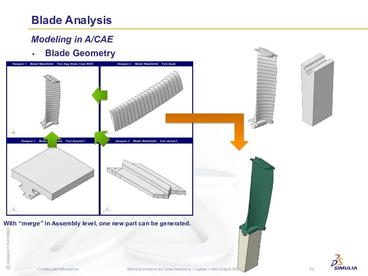
- 82. Blade Analysis Modeling in A/CAE Blade Geometry With “merge” in Assembly level, one new part can
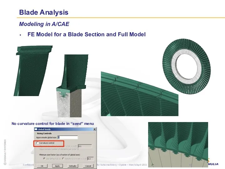
- 83. Blade Analysis Modeling in A/CAE FE Model for a Blade Section and Full Model No curvature
- 84. Blade Analysis Cyclic Symmetric Model Surface “slave” Surface “master” *SURFACE, NAME=master *SURFACE, NAME=slave *TIE, CYCLIC SYMMETRY,
- 85. Blade Analysis Modal Analysis Frequency extraction capability is supported with Lanczos solver only for cyclic symmetric
- 86. Blade Analysis Modal Analysis Frequency extraction capability is supported with Lanczos solver only for cyclic symmetric
- 87. Blade Analysis After mapping the temperature results from the previous analysis, stress analysis considering temperature and
- 88. Blade Analysis Stress Analysis Stress analysis after mapping temperature Temperature Mapping Area Temperature from CFD Applied
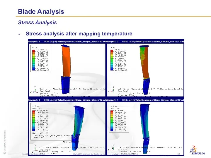
- 89. Blade Analysis Stress Analysis Stress analysis after mapping temperature
- 90. Blade Analysis Sources of the data can be (but are not limited to): A previous Abaqus
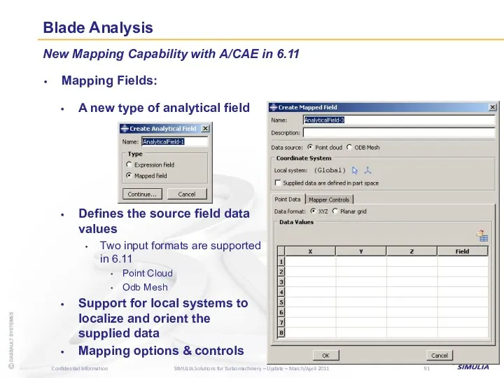
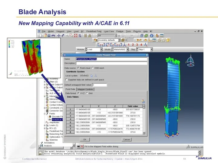
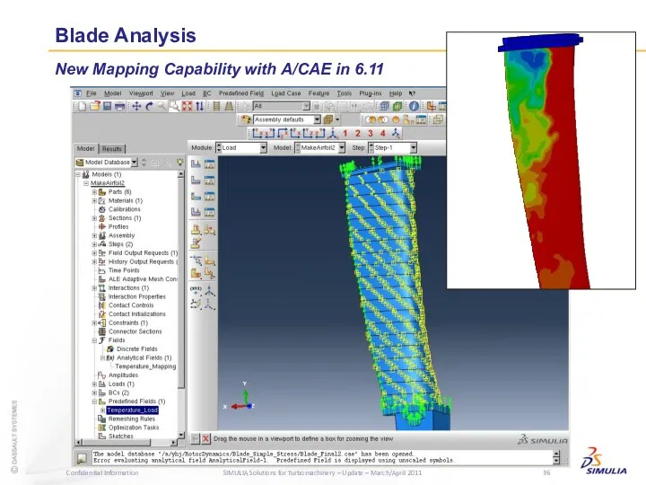
- 91. Blade Analysis Mapping Fields: New Mapping Capability with A/CAE in 6.11 A new type of analytical
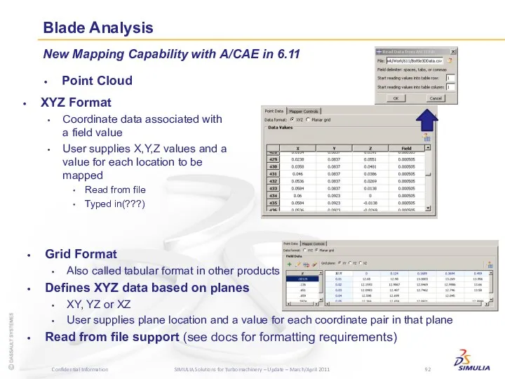
- 92. Blade Analysis Point Cloud New Mapping Capability with A/CAE in 6.11 XYZ Format Coordinate data associated
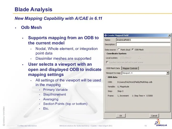
- 93. Blade Analysis Odb Mesh New Mapping Capability with A/CAE in 6.11 Supports mapping from an ODB
- 94. Blade Analysis New Mapping Capability with A/CAE in 6.11
- 95. Blade Analysis New Mapping Capability with A/CAE in 6.11
- 96. Blade Analysis New Mapping Capability with A/CAE in 6.11
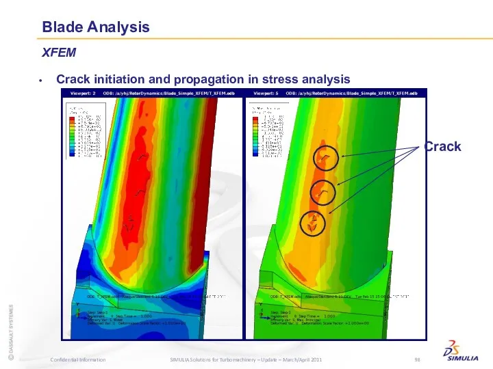
- 97. Blade Analysis XFEM Crack initiation and propagation in stress analysis Von Mises
- 98. Blade Analysis XFEM Crack initiation and propagation in stress analysis Crack
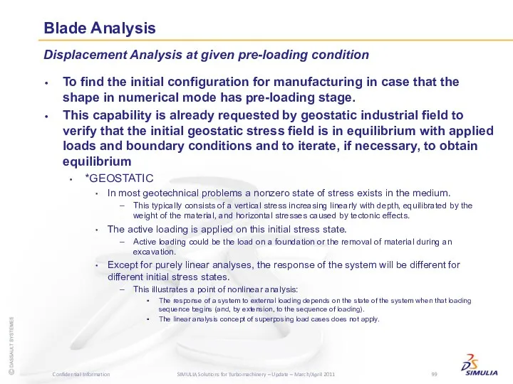
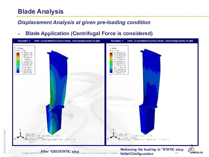
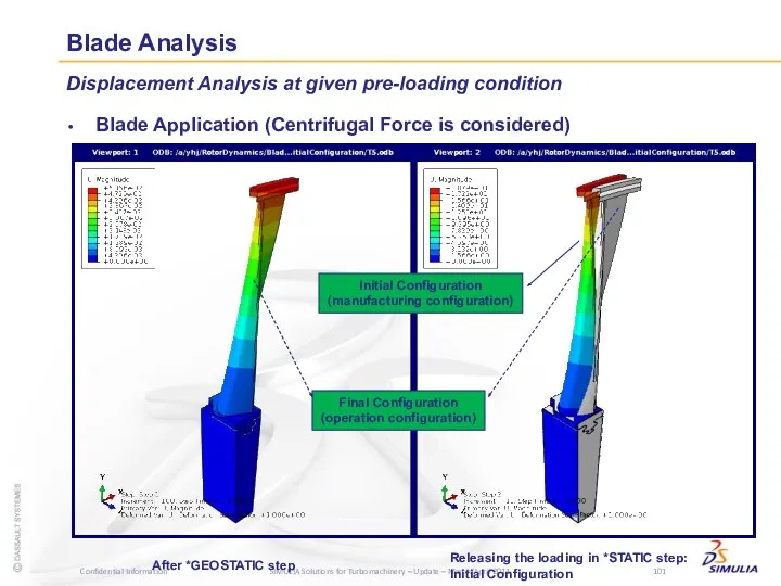
- 99. Blade Analysis To find the initial configuration for manufacturing in case that the shape in numerical
- 100. Blade Analysis Displacement Analysis at given pre-loading condition Blade Application (Centrifugal Force is considered) After *GEOSTATIC
- 101. Blade Analysis Displacement Analysis at given pre-loading condition Blade Application (Centrifugal Force is considered) After *GEOSTATIC
- 102. Blade-out Containment Analysis
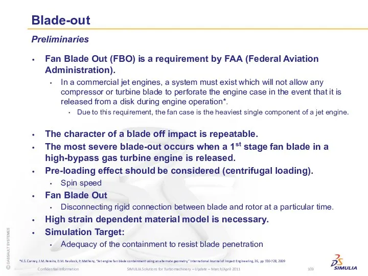
- 103. Blade-out Fan Blade Out (FBO) is a requirement by FAA (Federal Aviation Administration). In a commercial
- 104. Blade-out Model in reference* (Flat and Curved Plates) *K.S. Carney, J.M. Pereira, D.M. Revilock, P. Matheny,
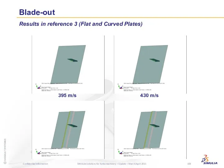
- 105. Blade-out Results in reference 3 (Flat and Curved Plates) 394 m/s 457m/s 430 m/s 490 m/s
- 106. Blade-out Abaqus result comparison for flat plate 394 m/s 457m/s * Need to adjust damage parameter
- 107. Blade-out Results in reference 3 (Flat and Curved Plates) 430 m/s 490 m/s
- 108. Blade-out Results in reference 3 (Flat and Curved Plates) 395 m/s 430 m/s
- 109. Blade-out Results in reference 3 (Flat and Curved Plates) LS-DYNA Abaqus
- 110. Blade-out Further Investigation for reference 3 (Flat and Curved Plates) Cross-section 21.17 mm 25.4 mm M1
- 111. Blade-out Further Investigation for reference 3 (Flat and Curved Plates) M1: 490 m/s M2: 490 m/s
- 112. Blade-out Further Investigation for reference 3 (Flat and Curved Plates) M1: 520 m/s M2: 520 m/s
- 113. Blade-out Further Investigation for containment (1000 rad/s spin speed) A/Explicit A/Standard Forced Failure Step 1 (Failure
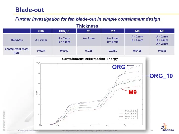
- 114. Blade-out Further Investigation for fan blade-out in simple containment design A A B A A B
- 115. Blade-out Further Investigation for fan blade-out in simple containment design ORG Flat with the same thickness
- 116. Blade-out Further Investigation for fan blade-out in simple containment design ORG Flat with the same thickness
- 117. Blade-out Further Investigation for fan blade-out in simple containment design ORG Flat with the same thickness
- 118. Blade-out Further Investigation for fan blade-out in simple containment design ORG_10 Flat with different thickness M9
- 119. Blade-out Further Investigation for fan blade-out in simple containment design M9 Tapered with the different thickness
- 120. Blade-out Further Investigation for fan blade-out in simple containment design Thickness M9 ORG ORG_10
- 121. Foreign Object Impact Analysis
- 122. Foreign Object Impact Analysis Bird Model: ANSWER 4493 Best Practices for Bird Strike Simulations with Abaqus/Explicit
- 123. Foreign Object Impact Analysis Lagrangian Approach
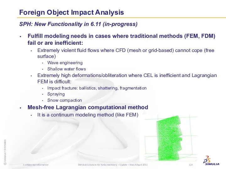
- 124. Foreign Object Impact Analysis Fulfill modeling needs in cases where traditional methods (FEM, FDM) fail or
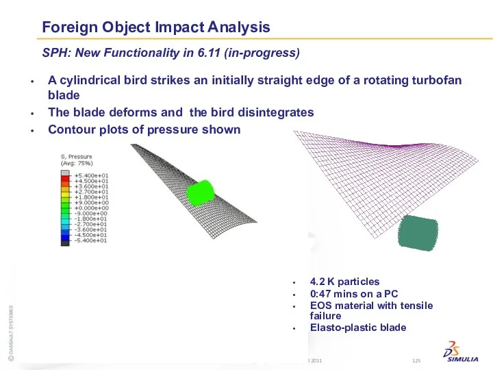
- 125. Foreign Object Impact Analysis SPH: New Functionality in 6.11 (in-progress) A cylindrical bird strikes an initially
- 127. Скачать презентацию
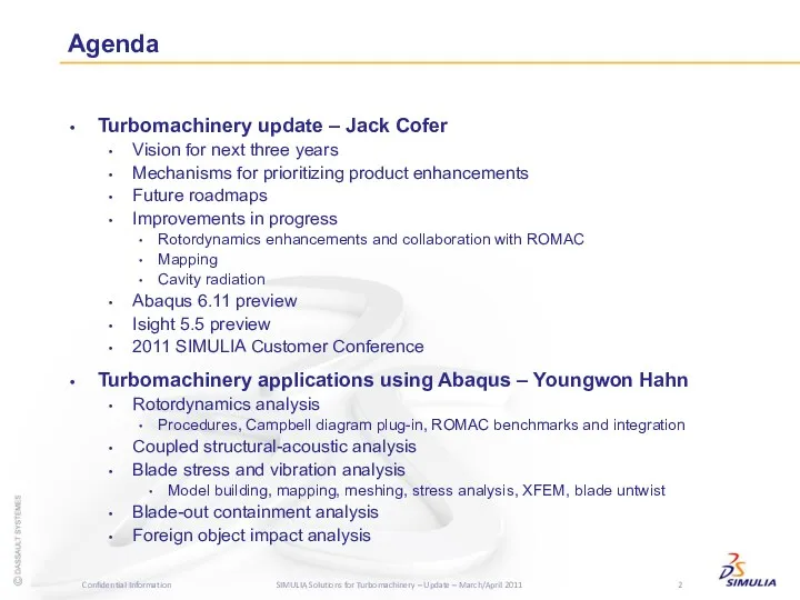
Agenda
Turbomachinery update – Jack Cofer
Vision for next three years
Mechanisms for prioritizing
Agenda
Turbomachinery update – Jack Cofer
Vision for next three years
Mechanisms for prioritizing

Agenda (Siemens)
Turbomachinery update – Jack Cofer
Vision for next three years
Future roadmaps
Improvements
Agenda (Siemens)
Turbomachinery update – Jack Cofer
Vision for next three years
Future roadmaps
Improvements
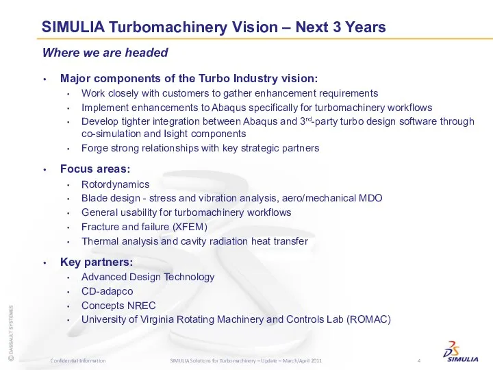
SIMULIA Turbomachinery Vision – Next 3 Years
Major components of the Turbo
SIMULIA Turbomachinery Vision – Next 3 Years
Major components of the Turbo

Mechanisms for Prioritizing Requests for Enhancements
Customers submit RFEs through their local
Mechanisms for Prioritizing Requests for Enhancements
Customers submit RFEs through their local
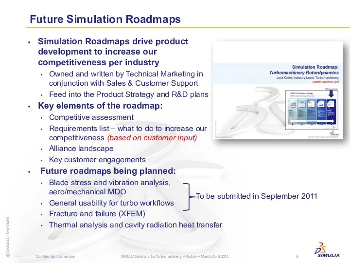
Future Simulation Roadmaps
Simulation Roadmaps drive product development to increase our competitiveness
Future Simulation Roadmaps
Simulation Roadmaps drive product development to increase our competitiveness
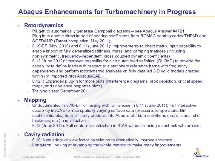
Rotordynamics
Plug-in to automatically generate Campbell diagrams – see Abaqus Answer #4721
Plug-in
Rotordynamics
Plug-in to automatically generate Campbell diagrams – see Abaqus Answer #4721
Plug-in
UVA Rotating Machinery and Controls Laboratory
(ROMAC) Industrial Program
In June 2010, SIMULIA
UVA Rotating Machinery and Controls Laboratory
(ROMAC) Industrial Program
In June 2010, SIMULIA

Joint Rotordynamics Work with ROMAC
Dr. Youngwon Hahn is currently working with
Joint Rotordynamics Work with ROMAC
Dr. Youngwon Hahn is currently working with

Major RFE Status (Siemens)
Mapping issues
Displaying contour plots of all loads/boundaries/fields (including
Major RFE Status (Siemens)
Mapping issues
Displaying contour plots of all loads/boundaries/fields (including
Abaqus 6.11 Preview
SIMULIA Technical Marketing
Abaqus 6.11 Preview
SIMULIA Technical Marketing
GPGPU Acceleration
Direct solver acceleration using GPGPU’s
Speed-ups of 2-3x have been observed
Benefits
GPGPU Acceleration
Direct solver acceleration using GPGPU’s
Speed-ups of 2-3x have been observed
Benefits
Suitable for large deformation problems involving damage/fragmentation
Increases competitiveness in aerospace and
Suitable for large deformation problems involving damage/fragmentation
Increases competitiveness in aerospace and
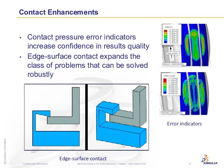
Contact pressure error indicators increase confidence in results quality
Edge-surface contact expands
Contact pressure error indicators increase confidence in results quality
Edge-surface contact expands
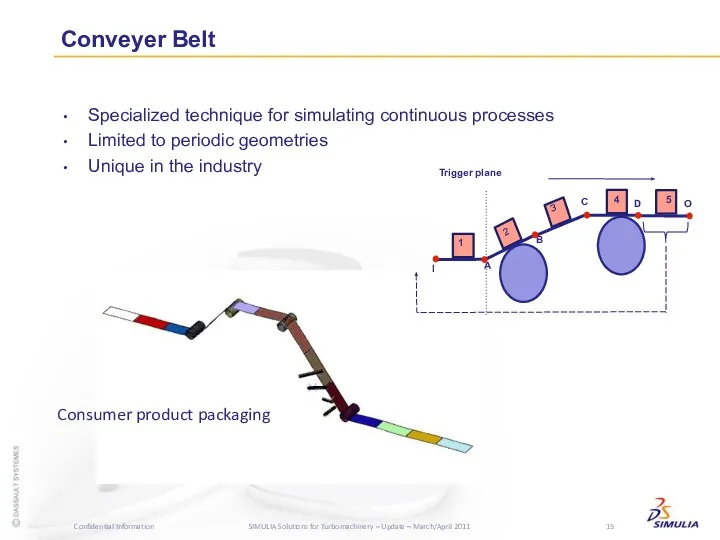
Conveyer Belt
Specialized technique for simulating continuous processes
Limited to periodic geometries
Unique in
Conveyer Belt
Specialized technique for simulating continuous processes
Limited to periodic geometries
Unique in

Parallel Frequency Response Solver
Targeted towards automotive NV market
Supports SMP w/ up
Parallel Frequency Response Solver
Targeted towards automotive NV market
Supports SMP w/ up
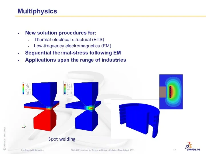
Multiphysics
New solution procedures for:
Thermal-electrical-structural (ETS)
Low-frequency electromagnetics (EM)
Sequential thermal-stress following EM
Applications
Multiphysics
New solution procedures for:
Thermal-electrical-structural (ETS)
Low-frequency electromagnetics (EM)
Sequential thermal-stress following EM
Applications
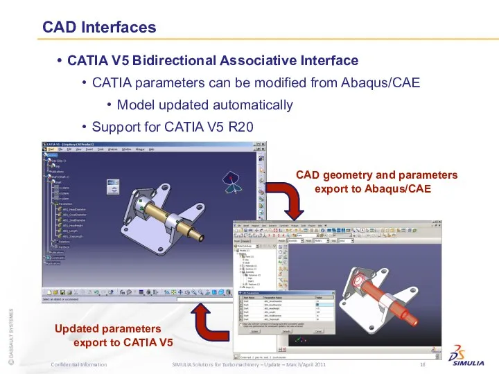
CATIA V5 Bidirectional Associative Interface
CATIA parameters can be modified from Abaqus/CAE
CATIA V5 Bidirectional Associative Interface
CATIA parameters can be modified from Abaqus/CAE
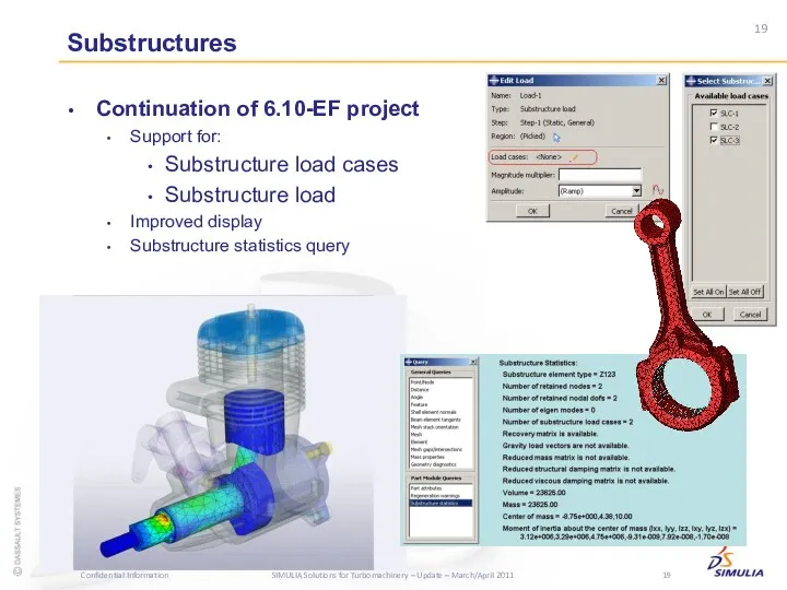
Substructures
Continuation of 6.10-EF project
Support for:
Substructure load cases
Substructure load
Improved display
Substructure statistics
Substructures
Continuation of 6.10-EF project
Support for:
Substructure load cases
Substructure load
Improved display
Substructure statistics

Reduce picking needed to create mid-surface
Improved robustness
Offset operation performance
Feature regeneration
Enhanced heuristics
Reduce picking needed to create mid-surface
Improved robustness
Offset operation performance
Feature regeneration
Enhanced heuristics
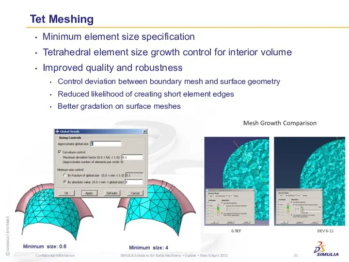
Tet Meshing
Minimum element size specification
Tetrahedral element size growth control for interior
Tet Meshing
Minimum element size specification
Tetrahedral element size growth control for interior
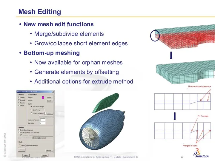
New mesh edit functions
Merge/subdivide elements
Grow/collapse short element edges
Bottom-up meshing
Now available
New mesh edit functions
Merge/subdivide elements
Grow/collapse short element edges
Bottom-up meshing
Now available
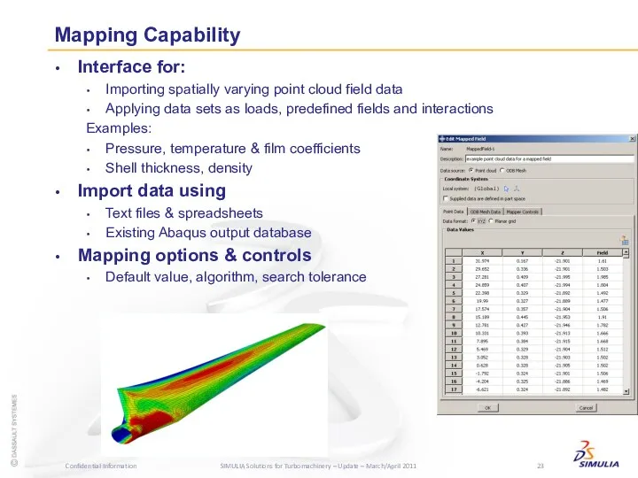
Mapping Capability
Interface for:
Importing spatially varying point cloud field data
Applying
Mapping Capability
Interface for:
Importing spatially varying point cloud field data
Applying
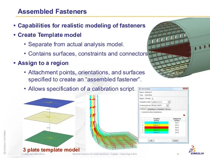
Capabilities for realistic modeling of fasteners
Create Template model
Separate from actual
Capabilities for realistic modeling of fasteners
Create Template model
Separate from actual
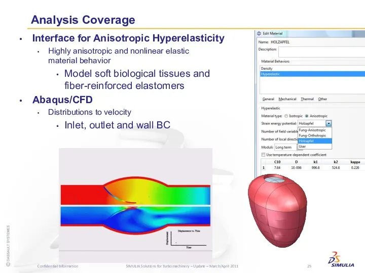
Analysis Coverage
Interface for Anisotropic Hyperelasticity
Highly anisotropic and nonlinear elastic
material behavior
Model
Analysis Coverage
Interface for Anisotropic Hyperelasticity
Highly anisotropic and nonlinear elastic
material behavior
Model
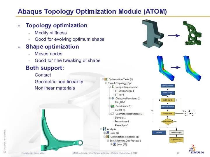
Abaqus Topology Optimization Module (ATOM)
Topology optimization
Modify stiffness
Good for evolving optimum shape
Shape
Abaqus Topology Optimization Module (ATOM)
Topology optimization
Modify stiffness
Good for evolving optimum shape
Shape
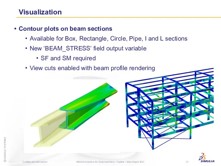
Contour plots on beam sections
Available for Box, Rectangle, Circle, Pipe, I
Contour plots on beam sections
Available for Box, Rectangle, Circle, Pipe, I

Section force/moment history output
Section force/moment display on multiple view cuts
Multiple free
Section force/moment history output
Section force/moment display on multiple view cuts
Multiple free

Isight 5.5 Preview
SIMULIA Technical Marketing
Isight 5.5 Preview
SIMULIA Technical Marketing
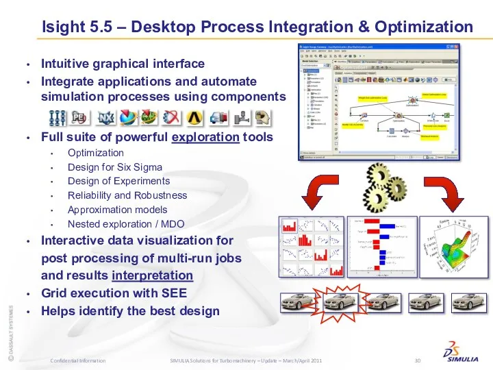
Intuitive graphical interface
Integrate applications and automate simulation processes using components
Full suite
Intuitive graphical interface
Integrate applications and automate simulation processes using components
Full suite
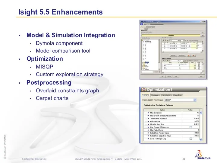
Isight 5.5 Enhancements
Model & Simulation Integration
Dymola component
Model comparison tool
Optimization
MISQP
Custom exploration strategy
Postprocessing
Overlaid
Isight 5.5 Enhancements
Model & Simulation Integration
Dymola component
Model comparison tool
Optimization
MISQP
Custom exploration strategy
Postprocessing
Overlaid

Isight 5.5 Enhancements: Model & Simulation Integration
Dymola Component allows users to
Isight 5.5 Enhancements: Model & Simulation Integration
Dymola Component allows users to
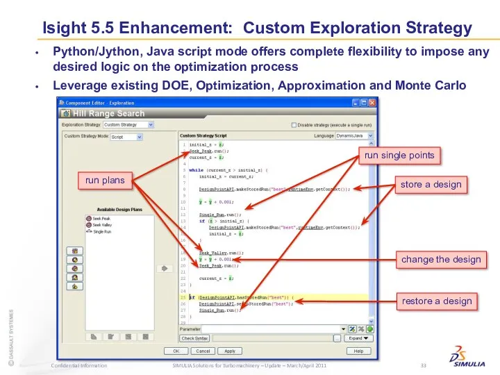
Python/Jython, Java script mode offers complete flexibility to impose any desired
Python/Jython, Java script mode offers complete flexibility to impose any desired
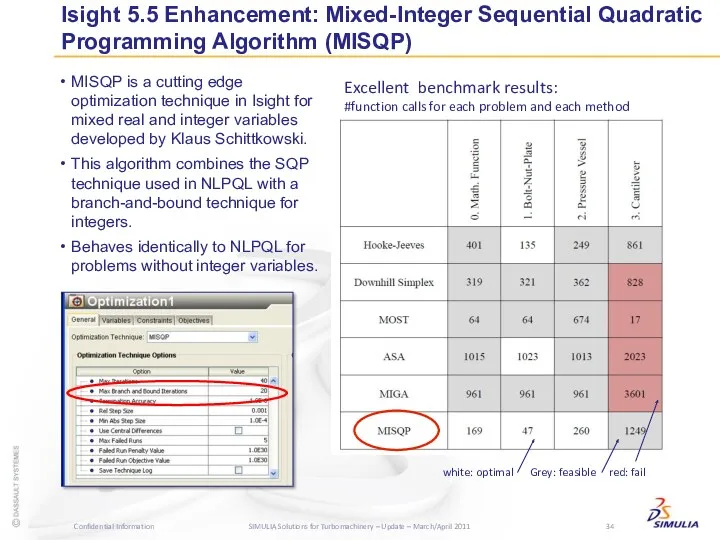
Isight 5.5 Enhancement: Mixed-Integer Sequential Quadratic Programming Algorithm (MISQP)
Excellent benchmark results:
Isight 5.5 Enhancement: Mixed-Integer Sequential Quadratic Programming Algorithm (MISQP)
Excellent benchmark results:

2011 SIMULIA Customer Conference
Advanced Seminars - May 16; Conference - May
2011 SIMULIA Customer Conference
Advanced Seminars - May 16; Conference - May
www.simulia.com/solutions/turbomachinery.html
New site still under development, new content added periodically
SIMULIA Customer Conference
www.simulia.com/solutions/turbomachinery.html
New site still under development, new content added periodically
SIMULIA Customer Conference
Turbomachinery Applications using Abaqus
Youngwon Hahn
Ver. OCT 2010
Turbomachinery Applications using Abaqus
Youngwon Hahn
Ver. OCT 2010
Who Is Dr. Youngwon Hahn?
Who Is Dr. Youngwon Hahn?
Overview
Rotordynamics
Gyroscopic Effect
Bearing Modeling
Frequency Extraction and Frequency Response
Campbell Diagram Plug-in
Other Plug-in in
Overview
Rotordynamics
Gyroscopic Effect
Bearing Modeling
Frequency Extraction and Frequency Response
Campbell Diagram Plug-in
Other Plug-in in
Rotordynamics
Rotordynamics

Rotordynamics
Abaqus provides two approaches for gyroscopic effect.
Eulerian approach
This technique was required
Rotordynamics
Abaqus provides two approaches for gyroscopic effect.
Eulerian approach
This technique was required

Rotordynamics
Lagrangian approach
General approach.
User can apply body force as the function of
Rotordynamics
Lagrangian approach
General approach.
User can apply body force as the function of
Rotordynamics
Bearing is a flexible component to support shaft.
Bearing has stiffness and
Rotordynamics
Bearing is a flexible component to support shaft.
Bearing has stiffness and
Rotordynamics
Real frequency extraction
Lanczos and AMS solver is supported.
AMS (Automatic Multi-level Substructuring)
Rotordynamics
Real frequency extraction
Lanczos and AMS solver is supported.
AMS (Automatic Multi-level Substructuring)
Rotordynamics
Rotational Loads
Defined by a prior SST Step
Unbalance Load Definition
Are assumed of
Rotordynamics
Rotational Loads
Defined by a prior SST Step
Unbalance Load Definition
Are assumed of
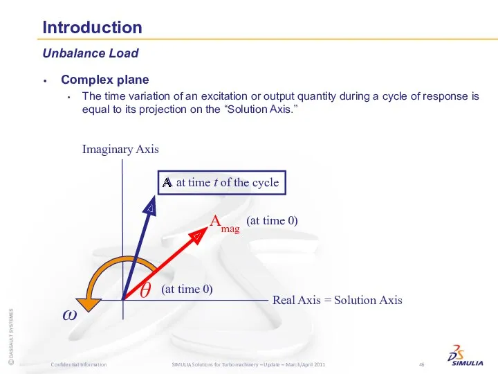
Introduction
Complex plane
The time variation of an excitation or output quantity during
Introduction
Complex plane
The time variation of an excitation or output quantity during

Rotordynamics
Complex axes to physical axes
Example: Unit force due to an
Rotordynamics
Complex axes to physical axes
Example: Unit force due to an

Rotordynamics
Use right-hand rule
To define 1-axis in the direction of real
Rotordynamics
Use right-hand rule
To define 1-axis in the direction of real
Rotordynamics
Example: Load
Rotordynamics
Example: Load
Rotordynamics
Comparison with reference paper
Frequency Extraction and Frequency Response
Reference Results*
*T.C. Gmur and
Rotordynamics
Comparison with reference paper
Frequency Extraction and Frequency Response
Reference Results*
*T.C. Gmur and
Rotordynamics
Comparison with reference paper
Frequency Extraction and Frequency Response
*T.C. Gmur and J.D.
Rotordynamics
Comparison with reference paper
Frequency Extraction and Frequency Response
*T.C. Gmur and J.D.
Rotordynamics
Comparison with analytical solution
Frequency Extraction and Frequency Response
Shaft assumed Massless, but
Rotordynamics
Comparison with analytical solution
Frequency Extraction and Frequency Response
Shaft assumed Massless, but

Rotordynamics
Comparison with analytical solution
Frequency Extraction and Frequency Response
*J.P. Den Hartog, “Mechanical
Rotordynamics
Comparison with analytical solution
Frequency Extraction and Frequency Response
*J.P. Den Hartog, “Mechanical
Rotordynamics
Comparison with ROMAC results
Shaft: L=50, Do=2, Di=0.1
Disk: L=2, Do=18, Di=2
Bearing location:
Rotordynamics
Comparison with ROMAC results
Shaft: L=50, Do=2, Di=0.1
Disk: L=2, Do=18, Di=2
Bearing location:

Rotordynamics
Comparison with ROMAC results
With uncoupled bearing (no Kxy/Kyx)
Kxx = 1000, Kzz
Rotordynamics
Comparison with ROMAC results
With uncoupled bearing (no Kxy/Kyx)
Kxx = 1000, Kzz
Rotordynamics
Comparison with ROMAC results
With uncoupled bearing (no Kxy/Kyx)
Kxx = 1000, Kzz
Rotordynamics
Comparison with ROMAC results
With uncoupled bearing (no Kxy/Kyx)
Kxx = 1000, Kzz
Rotordynamics
Comparison with ROMAC results
With uncoupled bearing (no Kxy/Kyx)
Kxx = 1000, Kzz
Rotordynamics
Comparison with ROMAC results
With uncoupled bearing (no Kxy/Kyx)
Kxx = 1000, Kzz
Rotordynamics
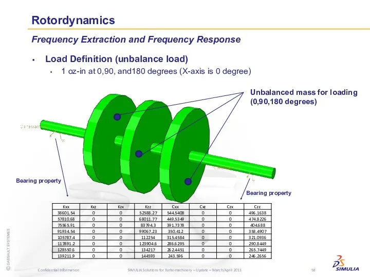
Load Definition (unbalance load)
1 oz-in at 0,90, and180 degrees (X-axis is
Rotordynamics
Load Definition (unbalance load)
1 oz-in at 0,90, and180 degrees (X-axis is

Simple Rotor (Three Disks)
Frequency Extraction and Frequency Response
Simple Rotor (Three Disks)
Frequency Extraction and Frequency Response

Rotordynamics
Newly developed A/Viewer Plug-in for rotordynamic application
Campbell Diagram Plug-in (ANSWER 4721)
Rotordynamics
Newly developed A/Viewer Plug-in for rotordynamic application
Campbell Diagram Plug-in (ANSWER 4721)
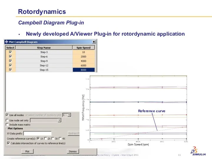
Rotordynamics
Newly developed A/Viewer Plug-in for rotordynamic application
Campbell Diagram Plug-in
Reference curve
Rotordynamics
Newly developed A/Viewer Plug-in for rotordynamic application
Campbell Diagram Plug-in
Reference curve
Rotordynamics
Plug-in to import bearing property from ROMAC Bearing Code (THBRG, THPAD,
Rotordynamics
Plug-in to import bearing property from ROMAC Bearing Code (THBRG, THPAD,

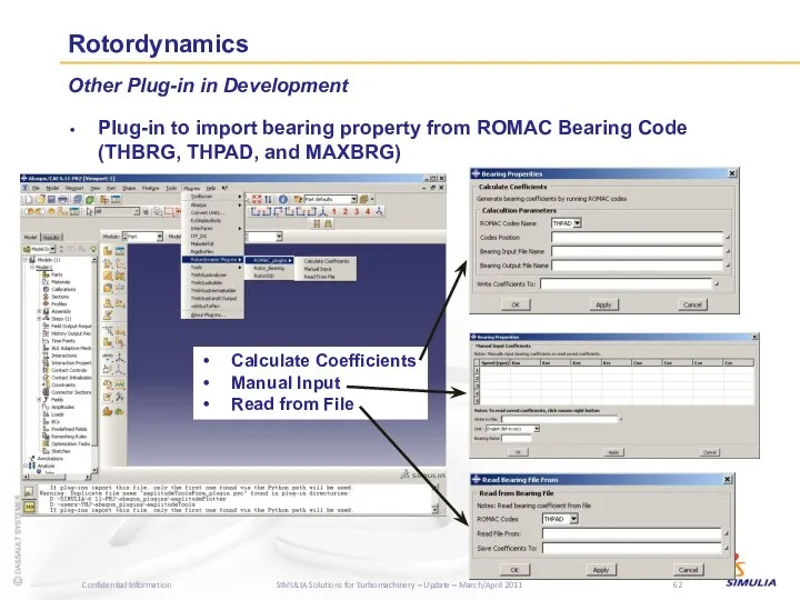
Rotordynamics
Plug-in to import bearing property from ROMAC Bearing Code (THBRG, THPAD,
Rotordynamics
Plug-in to import bearing property from ROMAC Bearing Code (THBRG, THPAD,

Rotordynamics
Plug-in to import bearing property from ROMAC Bearing Code (THBRG, THPAD,
Rotordynamics
Plug-in to import bearing property from ROMAC Bearing Code (THBRG, THPAD,

Rotordynamics
Plug-in to import bearing property from ROMAC Bearing Code (THBRG, THPAD,
Rotordynamics
Plug-in to import bearing property from ROMAC Bearing Code (THBRG, THPAD,
Rotordynamics
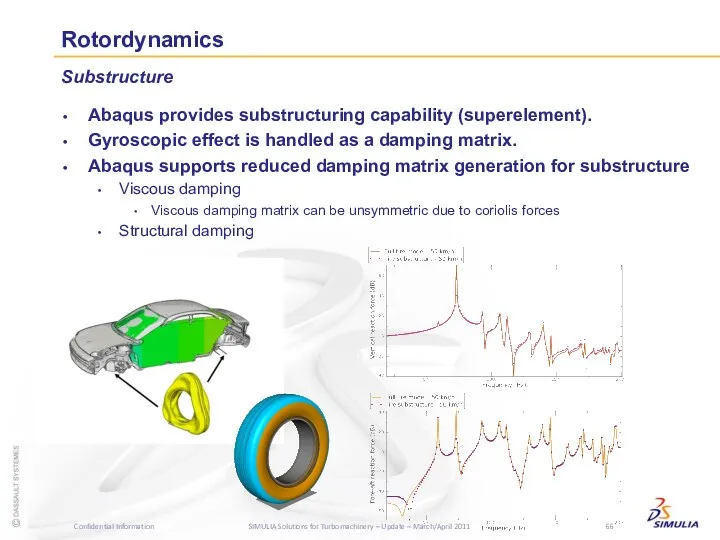
Abaqus provides substructuring capability (superelement).
Gyroscopic effect is handled as a damping
Rotordynamics
Abaqus provides substructuring capability (superelement).
Gyroscopic effect is handled as a damping

Rotordynamics
Example: Rotor-bearing system with support structure.
Modal analysis considering spin speed (261
Rotordynamics
Example: Rotor-bearing system with support structure.
Modal analysis considering spin speed (261
Rotordynamics
Rotor-bearing system with support structure.
Three different cases: full model, support substructure,
Rotordynamics
Rotor-bearing system with support structure.
Three different cases: full model, support substructure,

Rotordynamics
Rotor-bearing system with support structure.
Three different cases: full model, support substructure,
Rotordynamics
Rotor-bearing system with support structure.
Three different cases: full model, support substructure,
Rotordynamics
Rotor-bearing system with support structure (refined model)
Three different cases: full model,
Rotordynamics
Rotor-bearing system with support structure (refined model)
Three different cases: full model,
Rotordynamics
Rotor-bearing system with support structure.
Three different cases: full model, shaft substructures
Rotordynamics
Rotor-bearing system with support structure.
Three different cases: full model, shaft substructures
Coupled Structural-Acoustic Analysis
Coupled Structural-Acoustic Analysis

Coupled Structural-Acoustic Analysis
Lanczos and AMS solvers support coupled structural-acoustic analysis.
We have
Coupled Structural-Acoustic Analysis
Lanczos and AMS solvers support coupled structural-acoustic analysis.
We have
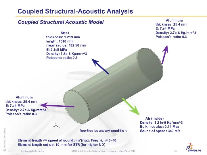
Coupled Structural-Acoustic Analysis
Coupled Structural Acoustic Model
Steel
thickness: 1.219 mm
length: 1010 mm
mean
Coupled Structural-Acoustic Analysis
Coupled Structural Acoustic Model
Steel
thickness: 1.219 mm
length: 1010 mm
mean
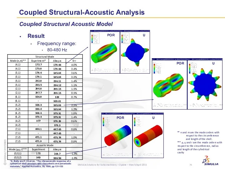
Coupled Structural-Acoustic Analysis
Coupled Structural Acoustic Model
Result
Frequency range:
80-480 Hz
*S. Boily and F.
Coupled Structural-Acoustic Analysis
Coupled Structural Acoustic Model
Result
Frequency range:
80-480 Hz
*S. Boily and F.

Blade Analysis
Blade Analysis
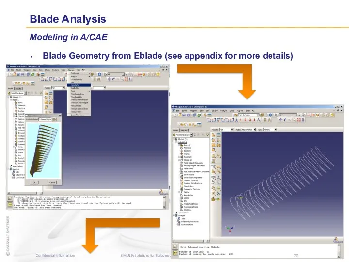
Blade Analysis
Blade Geometry from Eblade (see appendix for more details)
Modeling in
Blade Analysis
Blade Geometry from Eblade (see appendix for more details)
Modeling in

Blade Analysis
Import Eblade data to A/CAE: Plug-in
Number of section
Number of points
coordinates
The
Blade Analysis
Import Eblade data to A/CAE: Plug-in
Number of section
Number of points
coordinates
The
Blade Analysis
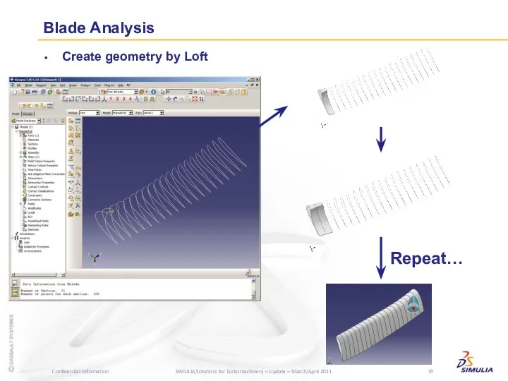
Create geometry by Loft
Repeat…
Blade Analysis
Create geometry by Loft
Repeat…
Blade Analysis
Meshing
Before meshing, do “combine edge” under “Virtual Topology” in “tool”
Blade Analysis
Meshing
Before meshing, do “combine edge” under “Virtual Topology” in “tool”
Blade Analysis
Meshing
Then, DO NOT check the curvature control in seed to
Blade Analysis
Meshing
Then, DO NOT check the curvature control in seed to
Blade Analysis
Modeling in A/CAE
Blade Geometry
With “merge” in Assembly level, one new
Blade Analysis
Modeling in A/CAE
Blade Geometry
With “merge” in Assembly level, one new
Blade Analysis
Modeling in A/CAE
FE Model for a Blade Section and Full
Blade Analysis
Modeling in A/CAE
FE Model for a Blade Section and Full
Blade Analysis
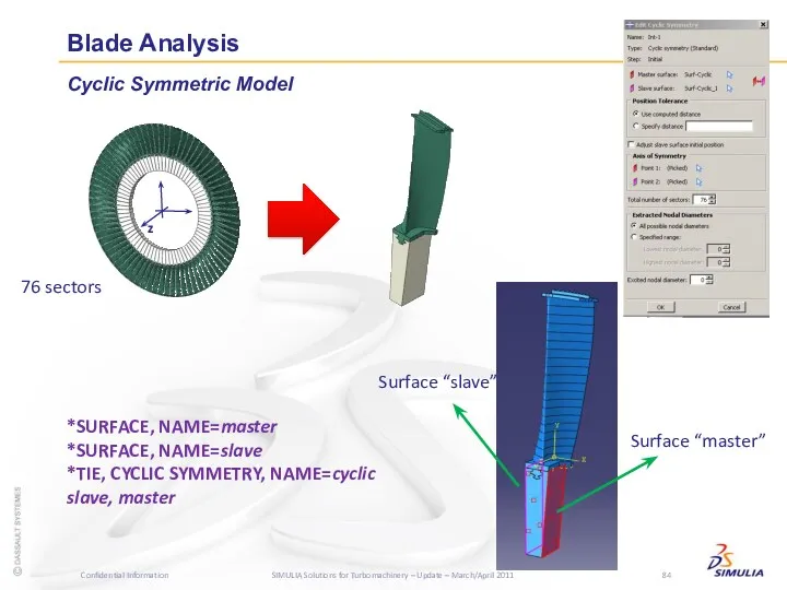
Cyclic Symmetric Model
Surface “slave”
Surface “master”
*SURFACE, NAME=master
*SURFACE, NAME=slave
*TIE, CYCLIC SYMMETRY, NAME=cyclic
slave,
Blade Analysis
Cyclic Symmetric Model
Surface “slave”
Surface “master”
*SURFACE, NAME=master
*SURFACE, NAME=slave
*TIE, CYCLIC SYMMETRY, NAME=cyclic
slave,
Blade Analysis
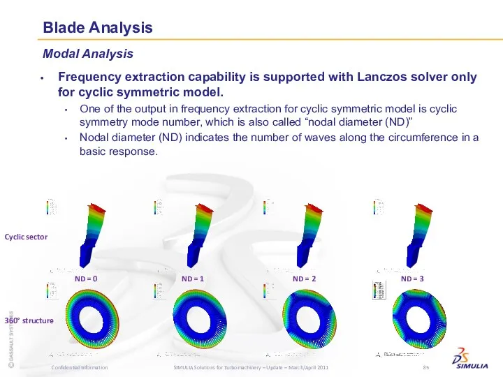
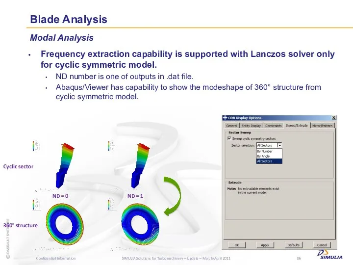
Modal Analysis
Frequency extraction capability is supported with Lanczos solver only
Blade Analysis
Modal Analysis
Frequency extraction capability is supported with Lanczos solver only
Blade Analysis
Modal Analysis
Frequency extraction capability is supported with Lanczos solver only
Blade Analysis
Modal Analysis
Frequency extraction capability is supported with Lanczos solver only

Blade Analysis
After mapping the temperature results from the previous analysis, stress
Blade Analysis
After mapping the temperature results from the previous analysis, stress
Blade Analysis
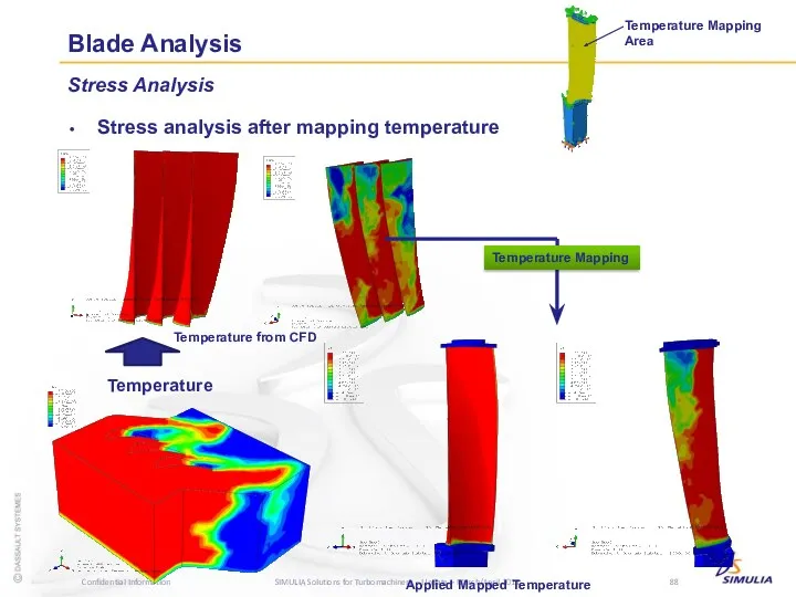
Stress Analysis
Stress analysis after mapping temperature
Temperature Mapping
Area
Temperature from CFD
Applied Mapped
Blade Analysis
Stress Analysis
Stress analysis after mapping temperature
Temperature Mapping
Area
Temperature from CFD
Applied Mapped
Blade Analysis
Stress Analysis
Stress analysis after mapping temperature
Blade Analysis
Stress Analysis
Stress analysis after mapping temperature

Blade Analysis
Sources of the data can be (but are not limited
Blade Analysis
Sources of the data can be (but are not limited
Blade Analysis
Mapping Fields:
New Mapping Capability with A/CAE in 6.11
A new type
Blade Analysis
Mapping Fields:
New Mapping Capability with A/CAE in 6.11
A new type
Blade Analysis
Point Cloud
New Mapping Capability with A/CAE in 6.11
XYZ Format
Coordinate data
Blade Analysis
Point Cloud
New Mapping Capability with A/CAE in 6.11
XYZ Format
Coordinate data
Blade Analysis
Odb Mesh
New Mapping Capability with A/CAE in 6.11
Supports mapping from
Blade Analysis
Odb Mesh
New Mapping Capability with A/CAE in 6.11
Supports mapping from
Blade Analysis
New Mapping Capability with A/CAE in 6.11
Blade Analysis
New Mapping Capability with A/CAE in 6.11

Blade Analysis
New Mapping Capability with A/CAE in 6.11
Blade Analysis
New Mapping Capability with A/CAE in 6.11
Blade Analysis
New Mapping Capability with A/CAE in 6.11
Blade Analysis
New Mapping Capability with A/CAE in 6.11

Blade Analysis
XFEM
Crack initiation and propagation in stress analysis
Von Mises
Blade Analysis
XFEM
Crack initiation and propagation in stress analysis
Von Mises
Blade Analysis
XFEM
Crack initiation and propagation in stress analysis
Crack
Blade Analysis
XFEM
Crack initiation and propagation in stress analysis
Crack
Blade Analysis
To find the initial configuration for manufacturing in case that
Blade Analysis
To find the initial configuration for manufacturing in case that
Blade Analysis
Displacement Analysis at given pre-loading condition
Blade Application (Centrifugal Force is
Blade Analysis
Displacement Analysis at given pre-loading condition
Blade Application (Centrifugal Force is
Blade Analysis
Displacement Analysis at given pre-loading condition
Blade Application (Centrifugal Force is
Blade Analysis
Displacement Analysis at given pre-loading condition
Blade Application (Centrifugal Force is

Blade-out Containment Analysis
Blade-out Containment Analysis
Blade-out
Fan Blade Out (FBO) is a requirement by FAA (Federal Aviation
Blade-out
Fan Blade Out (FBO) is a requirement by FAA (Federal Aviation

Blade-out
Model in reference* (Flat and Curved Plates)
*K.S. Carney, J.M. Pereira, D.M.
Blade-out
Model in reference* (Flat and Curved Plates)
*K.S. Carney, J.M. Pereira, D.M.

Blade-out
Results in reference 3 (Flat and Curved Plates)
394 m/s
457m/s
430 m/s
490 m/s
Flat
Blade-out
Results in reference 3 (Flat and Curved Plates)
394 m/s
457m/s
430 m/s
490 m/s
Flat

Blade-out
Abaqus result comparison for flat plate
394 m/s
457m/s
* Need to adjust damage
Blade-out
Abaqus result comparison for flat plate
394 m/s
457m/s
* Need to adjust damage

Blade-out
Results in reference 3 (Flat and Curved Plates)
430 m/s
490 m/s
Blade-out
Results in reference 3 (Flat and Curved Plates)
430 m/s
490 m/s
Blade-out
Results in reference 3 (Flat and Curved Plates)
395 m/s
430 m/s
Blade-out
Results in reference 3 (Flat and Curved Plates)
395 m/s
430 m/s
Blade-out
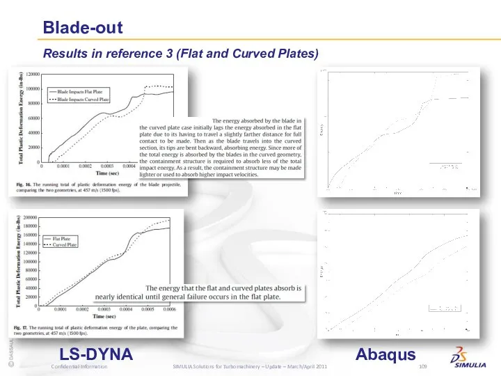
Results in reference 3 (Flat and Curved Plates)
LS-DYNA
Abaqus
Blade-out
Results in reference 3 (Flat and Curved Plates)
LS-DYNA
Abaqus
Blade-out
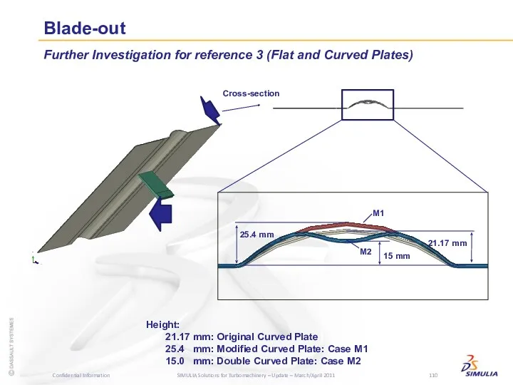
Further Investigation for reference 3 (Flat and Curved Plates)
Cross-section
21.17 mm
25.4 mm
M1
M2
Height:
21.17
Blade-out
Further Investigation for reference 3 (Flat and Curved Plates)
Cross-section
21.17 mm
25.4 mm
M1
M2
Height:
21.17
Blade-out
Further Investigation for reference 3 (Flat and Curved Plates)
M1: 490 m/s
M2:
Blade-out
Further Investigation for reference 3 (Flat and Curved Plates)
M1: 490 m/s
M2:

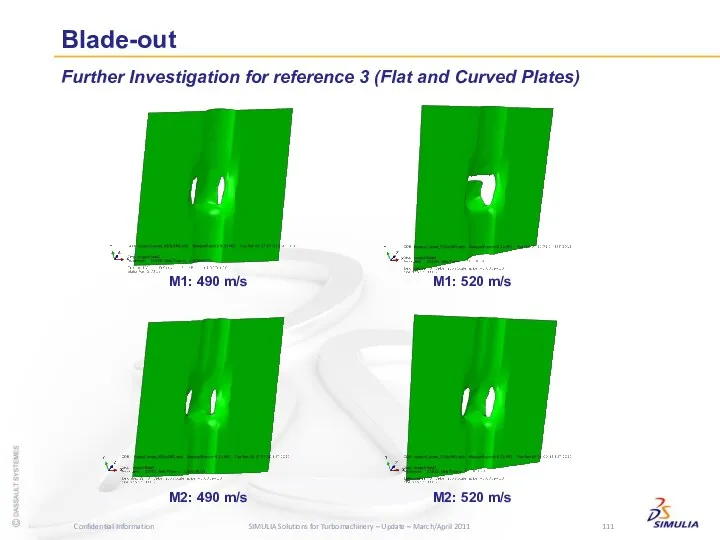
Blade-out
Further Investigation for reference 3 (Flat and Curved Plates)
M1: 520 m/s
M2:
Blade-out
Further Investigation for reference 3 (Flat and Curved Plates)
M1: 520 m/s
M2:

Blade-out
Further Investigation for containment (1000 rad/s spin speed)
A/Explicit
A/Standard
Forced Failure
Step 1
(Failure on
Blade-out
Further Investigation for containment (1000 rad/s spin speed)
A/Explicit
A/Standard
Forced Failure
Step 1
(Failure on
Blade-out
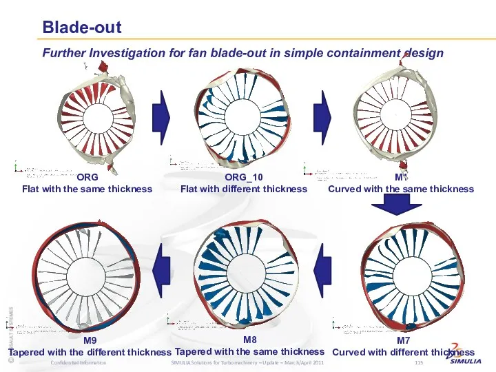
Further Investigation for fan blade-out in simple containment design
A
A
B
A
A
B
A
C
B
A
B
Blade-out
Further Investigation for fan blade-out in simple containment design
A
A
B
A
A
B
A
C
B
A
B
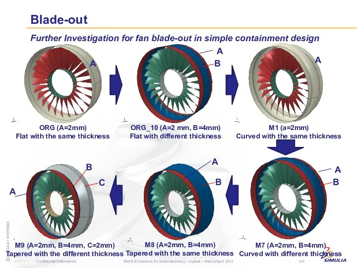
Blade-out
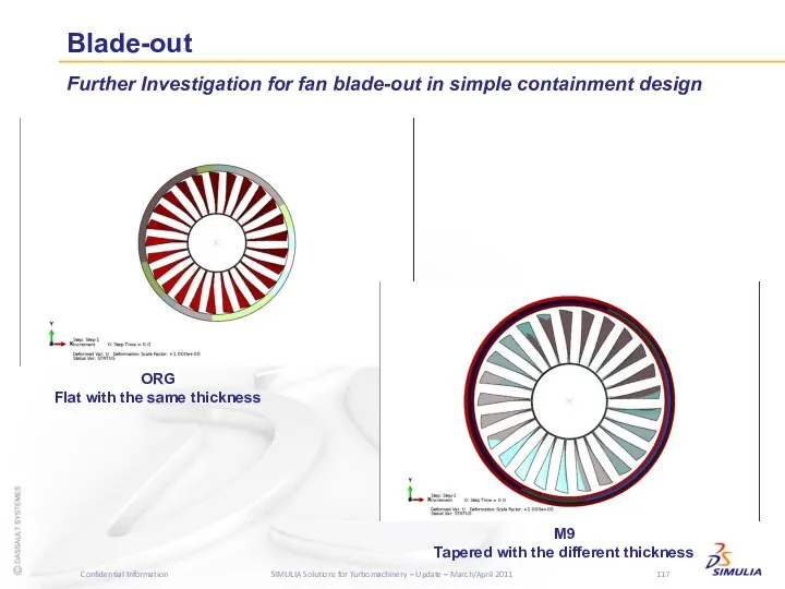
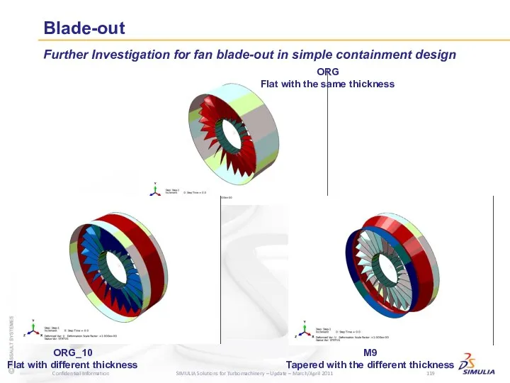
Further Investigation for fan blade-out in simple containment design
ORG
Flat with the
Blade-out
Further Investigation for fan blade-out in simple containment design
ORG
Flat with the

Blade-out
Further Investigation for fan blade-out in simple containment design
ORG
Flat with the
Blade-out
Further Investigation for fan blade-out in simple containment design
ORG
Flat with the
Blade-out
Further Investigation for fan blade-out in simple containment design
ORG
Flat with the
Blade-out
Further Investigation for fan blade-out in simple containment design
ORG
Flat with the
Blade-out
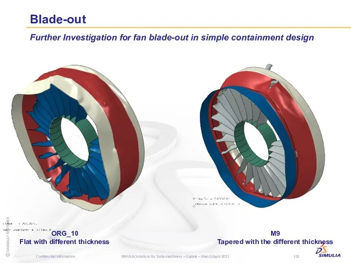
Further Investigation for fan blade-out in simple containment design
ORG_10
Flat with different
Blade-out
Further Investigation for fan blade-out in simple containment design
ORG_10
Flat with different
Blade-out
Further Investigation for fan blade-out in simple containment design
M9
Tapered with the
Blade-out
Further Investigation for fan blade-out in simple containment design
M9
Tapered with the
Blade-out
Further Investigation for fan blade-out in simple containment design
Thickness
M9
ORG
ORG_10
Blade-out
Further Investigation for fan blade-out in simple containment design
Thickness
M9
ORG
ORG_10

Foreign Object Impact Analysis
Foreign Object Impact Analysis

Foreign Object Impact Analysis
Bird Model: ANSWER 4493 Best Practices for Bird
Foreign Object Impact Analysis
Bird Model: ANSWER 4493 Best Practices for Bird

Foreign Object Impact Analysis
Lagrangian Approach
Foreign Object Impact Analysis
Lagrangian Approach
Foreign Object Impact Analysis
Fulfill modeling needs in cases where traditional methods
Foreign Object Impact Analysis
Fulfill modeling needs in cases where traditional methods
Foreign Object Impact Analysis
SPH: New Functionality in 6.11 (in-progress)
A cylindrical bird
Foreign Object Impact Analysis
SPH: New Functionality in 6.11 (in-progress)
A cylindrical bird
 Инструкция для подачи обращения/заявления для получения муниципальной услуги Зачисление в образовательное учреждение
 Динамические структуры данных. Указатели
 Centre Monitoring System PH-BC911 (Operation)
 LI-FI световая замена WI-FI
 CoDeSys - общий обзор
 Мастер-класс Получение услуг через Портал государственных и муниципальных услуг
 Плюсы и минусы информационного общества
 Алгоритм и его свойства. Понятие алгоритма и исполнителя. Свойства алгоритма
 Огляд введення та виведення в С++
 Филатов Андрей В-45
 Безопасность детей в интернете
 Логические основы построения компьютера
 Cистемы электронного документооборота
 Ведение базы данных в MS Access. Технологии баз данных. (Лекция 5)
 Компьютер как средство автоматизации информационных процессов.
 Рабочий стол. Управление мышью
 Верификация программного обеспечения. Дефекты
 Понятие юзабилити
 Файлы и файловые структуры. Компьютер как универсальное устройство для работы с информацией. Информатика. 7 класс
 Орта мектепте химия пәнінен типтік есептер шығаруда ақпараттық технологияны қолдану әдістері
 Современные информационные технологии в образовании
 Разработка web-сайта для ООО Лидер
 Искусственный интеллект, данные и знания. Экспертные системы. Лекция №1
 Информационные модели на графах
 Лекция 1. Системы обработки информации в таможенных органах Российской Федерации
 Кодирование информации
 MVC в Android. Создание простейшего приложения
 Разновидности объектов и их классификация