- Chapter 3. Polynomial and Rational Functions. 3.2 Polynomial Functions and Their Graphs

Содержание
- 2. Identify polynomial functions. Recognize characteristics of graphs of polynomial functions. Determine end behavior. Use factoring to
- 3. Definition of a Polynomial Function Let n be a nonnegative integer and let be real numbers,
- 4. Graphs of Polynomial Functions – Smooth and Continuous Polynomial functions of degree 2 or higher have
- 5. End Behavior of Polynomial Functions The end behavior of the graph of a function to the
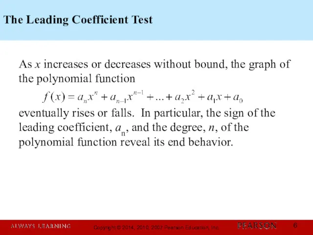
- 6. The Leading Coefficient Test As x increases or decreases without bound, the graph of the polynomial
- 7. The Leading Coefficient Test for (continued)
- 8. Example: Using the Leading Coefficient Test Use the Leading Coefficient Test to determine the end behavior
- 9. Zeros of Polynomial Functions If f is a polynomial function, then the values of x for
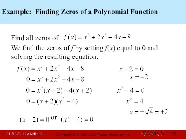
- 10. Example: Finding Zeros of a Polynomial Function Find all zeros of We find the zeros of
- 11. Example: Finding Zeros of a Polynomial Function (continued) Find all zeros of The zeros of f
- 12. Multiplicity and x-Intercepts If r is a zero of even multiplicity, then the graph touches the
- 13. Example: Finding Zeros and Their Multiplicities Find the zeros of and give the multiplicities of each
- 14. Example: Finding Zeros and Their Multiplicities (continued) We find the zeros of f by setting f(x)
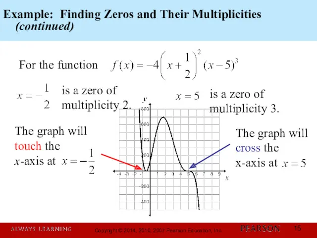
- 15. Example: Finding Zeros and Their Multiplicities (continued) For the function is a zero of multiplicity 2.
- 16. The Intermediate Value Theorem Let f be a polynomial function with real coefficients. If f(a) and
- 17. Example: Using the Intermediate Value Theorem Show that the polynomial function has a real zero between
- 18. Example: Using the Intermediate Value Theorem (continued) For f(–3) = –42 and f(–2) = 5. The
- 19. Turning Points of Polynomial Functions In general, if f is a polynomial function of degree n,
- 20. A Strategy for Graphing Polynomial Functions
- 21. Example: Graphing a Polynomial Function Use the five-step strategy to graph Step 1 Determine end behavior
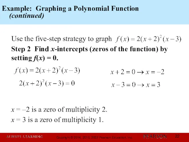
- 22. Example: Graphing a Polynomial Function (continued) Use the five-step strategy to graph Step 2 Find x-intercepts
- 23. Example: Graphing a Polynomial Function (continued) Use the five-step strategy to graph Step 2 (continued) Find
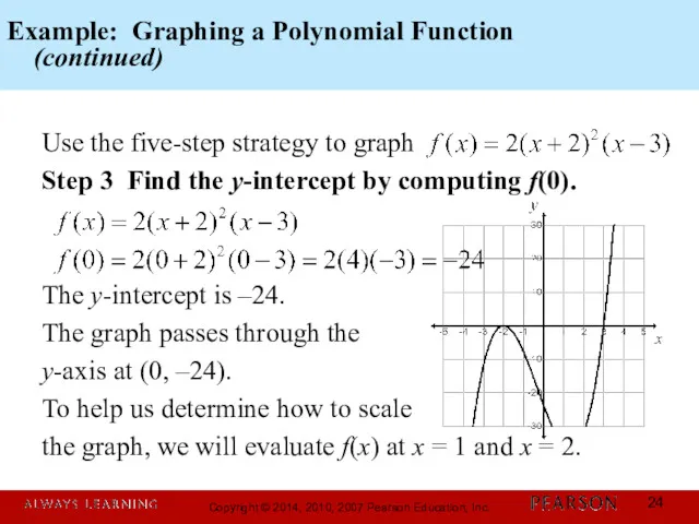
- 24. Example: Graphing a Polynomial Function (continued) Use the five-step strategy to graph Step 3 Find the
- 25. Example: Graphing a Polynomial Function (continued) Use the five-step strategy to graph Step 3 (continued) Find
- 26. Example: Graphing a Polynomial Function (continued) Use the five-step strategy to graph Step 4 Use possible
- 27. Example: Graphing a Polynomial Function (continued) Use the five-step strategy to graph Step 4 (continued) Use
- 29. Скачать презентацию

Identify polynomial functions.
Recognize characteristics of graphs of polynomial functions.
Determine end behavior.
Use
Identify polynomial functions.
Recognize characteristics of graphs of polynomial functions.
Determine end behavior.
Use

Definition of a Polynomial Function
Let n be a nonnegative integer and
Definition of a Polynomial Function
Let n be a nonnegative integer and

Graphs of Polynomial Functions – Smooth and Continuous
Polynomial functions of degree
Graphs of Polynomial Functions – Smooth and Continuous
Polynomial functions of degree

End Behavior of Polynomial Functions
The end behavior of the graph of
End Behavior of Polynomial Functions
The end behavior of the graph of
The Leading Coefficient Test
As x increases or decreases without bound, the
The Leading Coefficient Test
As x increases or decreases without bound, the

The Leading Coefficient Test for
(continued)
The Leading Coefficient Test for
(continued)

Example: Using the Leading Coefficient Test
Use the Leading Coefficient Test to
Example: Using the Leading Coefficient Test
Use the Leading Coefficient Test to

Zeros of Polynomial Functions
If f is a polynomial function, then the
Zeros of Polynomial Functions
If f is a polynomial function, then the
Example: Finding Zeros of a Polynomial Function
Find all zeros of
We
Example: Finding Zeros of a Polynomial Function
Find all zeros of
We

Example: Finding Zeros of a Polynomial Function
(continued)
Find all zeros of
The
Example: Finding Zeros of a Polynomial Function
(continued)
Find all zeros of
The

Multiplicity and x-Intercepts
If r is a zero of even multiplicity, then
Multiplicity and x-Intercepts
If r is a zero of even multiplicity, then

Example: Finding Zeros and Their Multiplicities
Find the zeros of
and give
Example: Finding Zeros and Their Multiplicities
Find the zeros of
and give

Example: Finding Zeros and Their Multiplicities
(continued)
We find the zeros of
Example: Finding Zeros and Their Multiplicities
(continued)
We find the zeros of
Example: Finding Zeros and Their Multiplicities
(continued)
For the function
is a
Example: Finding Zeros and Their Multiplicities
(continued)
For the function
is a

The Intermediate Value Theorem
Let f be a polynomial function with real
The Intermediate Value Theorem
Let f be a polynomial function with real

Example: Using the Intermediate Value Theorem
Show that the polynomial function
has a
Example: Using the Intermediate Value Theorem
Show that the polynomial function
has a

Example: Using the Intermediate Value Theorem
(continued)
For
f(–3) = –42
and
Example: Using the Intermediate Value Theorem
(continued)
For
f(–3) = –42
and

Turning Points of Polynomial Functions
In general, if f is a polynomial
Turning Points of Polynomial Functions
In general, if f is a polynomial
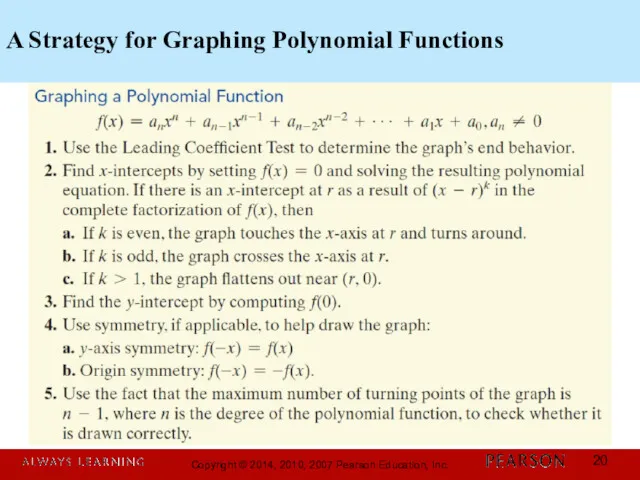
A Strategy for Graphing Polynomial Functions
A Strategy for Graphing Polynomial Functions

Example: Graphing a Polynomial Function
Use the five-step strategy to graph
Step 1
Example: Graphing a Polynomial Function
Use the five-step strategy to graph
Step 1
Example: Graphing a Polynomial Function
(continued)
Use the five-step strategy to graph
Step
Example: Graphing a Polynomial Function
(continued)
Use the five-step strategy to graph
Step

Example: Graphing a Polynomial Function
(continued)
Use the five-step strategy to graph
Step
Example: Graphing a Polynomial Function
(continued)
Use the five-step strategy to graph
Step
Example: Graphing a Polynomial Function
(continued)
Use the five-step strategy to graph
Step
Example: Graphing a Polynomial Function
(continued)
Use the five-step strategy to graph
Step

Example: Graphing a Polynomial Function
(continued)
Use the five-step strategy to graph
Step
Example: Graphing a Polynomial Function
(continued)
Use the five-step strategy to graph
Step

Example: Graphing a Polynomial Function
(continued)
Use the five-step strategy to graph
Step
Example: Graphing a Polynomial Function
(continued)
Use the five-step strategy to graph
Step

Example: Graphing a Polynomial Function
(continued)
Use the five-step strategy to graph
Step
Example: Graphing a Polynomial Function
(continued)
Use the five-step strategy to graph
Step
 Представление рациональных чисел в виде десятичной дроби (продолжение)
 Конспект и презентация к уроку-путешествию в лес, математика 1 класс Закрепление навыков сложения и вычитания в пределах 20
 Умножение натуральных чисел и его свойства. 5 класс
 Арифметическая игра Числовые Домики
 Умножение и деление обыкновенных дробей
 Смешанные числа. Обыкновенные дроби. Математика. 5 класс
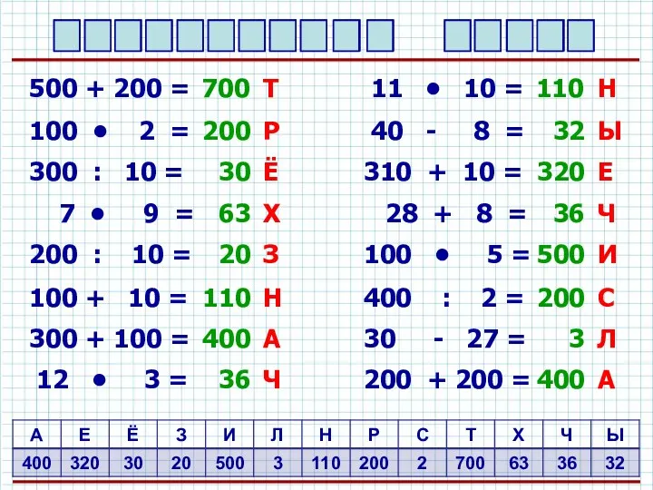 Сложение и вычитание трёхзначных чисел Презентация к уроку математики 3 класс
 Деление (математика, 3 класс, УМК Гармония)
 Презентация Времена года
 ЦМР к уроку математики в 1 классе Дециметр - новая единица длины
 Признаки делимости на 10, на 5 и на 2
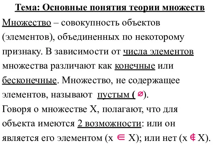 Множества и матрицы
 Презентация Веселая математика с Винни-Пухом
 Площадь треугольника
 Двузначные числа
 Решение задач с помощью кругов Эйлера
 Десятичные дроби и действия над ними
 Окружность. Касательная к окружности
 Распределительное свойство умножения
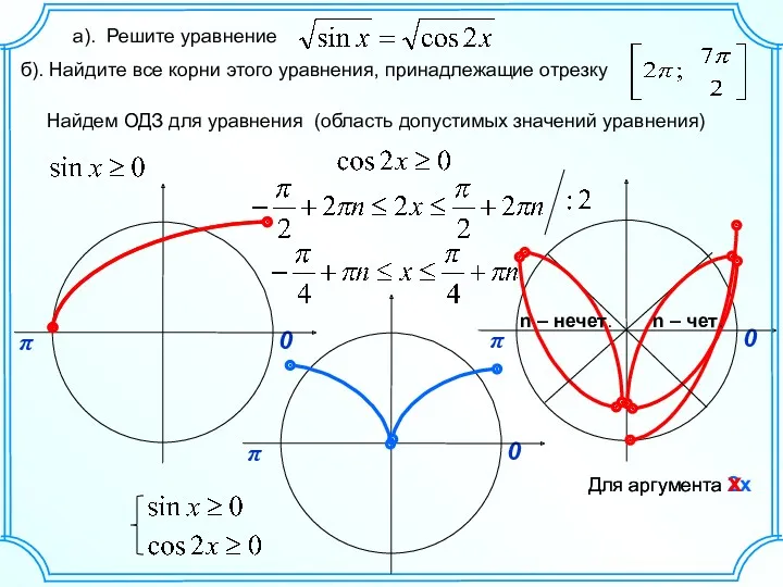 Решение тригонометрического уравнения (С 1, 26)
 Методические разработки учителя математики
 Скорость. Время. Расстояние
 Презентация к уроку математики в 4 классе.
 презентация к уроку математики Решение задач на движение
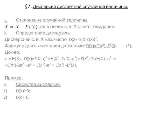 Дисперсия дискретной случайной величины
 Экономические задачи в заданиях ЕГЭ по математике
 Приёмы устных вычислений вида 450+30; 620-200
 Сложение и вычитание десятичных дробей. Урок 111