- Descriptive statistics

Содержание
- 2. Frequency Distributions and Their Graphs Section 2.1
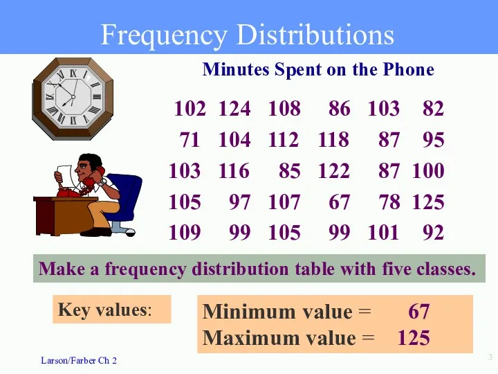
- 3. Frequency Distributions 102 124 108 86 103 82 71 104 112 118 87 95 103 116
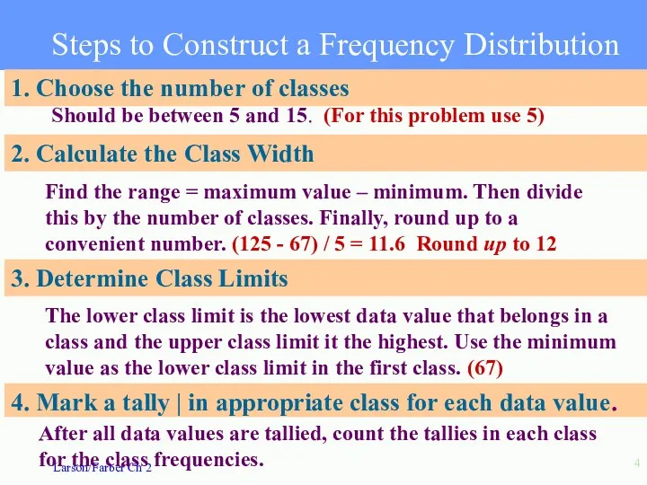
- 4. 4. Mark a tally | in appropriate class for each data value. Steps to Construct a
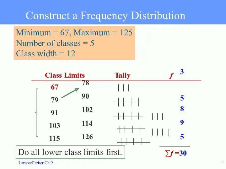
- 5. 78 90 102 114 126 3 5 8 9 5 67 79 91 103 115 Do
- 6. Boundaries 66.5 - 78.5 78.5 - 90.5 90.5 - 102.5 102.5 -114.5 114.5 -126.5 Frequency Histogram
- 7. Frequency Polygon Time on Phone minutes f Mark the midpoint at the top of each bar.
- 8. 67 - 78 79 - 90 91 - 102 103 -114 115 -126 3 5 8
- 9. Relative Frequency Histogram Time on Phone minutes Relative frequency Relative frequency on vertical scale
- 10. Ogive An ogive reports the number of values in the data set that are less than
- 11. More Graphs and Displays Section 2.2
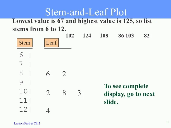
- 12. Stem-and-Leaf Plot 6 | 7 | 8 | 9 | 10| 11| 12| Lowest value is
- 13. 6 | 7 7 | 1 8 8 | 2 5 6 7 7 9 |
- 14. Stem-and-Leaf with two lines per stem 6 | 7 7 | 1 7 | 8 8
- 15. Dotplot 66 76 86 96 106 116 126 Phone minutes
- 16. NASA budget (billions of $) divided among 3 categories. Pie Chart Used to describe parts of
- 17. Total Pie Chart Billions of $ Human Space Flight 5.7 Technology 5.9 Mission Support 2.7 14.3
- 18. Scatter Plot x y 8 78 2 92 5 90 12 58 15 43 9 74
- 19. Measures of Central Tendency Section 2.3
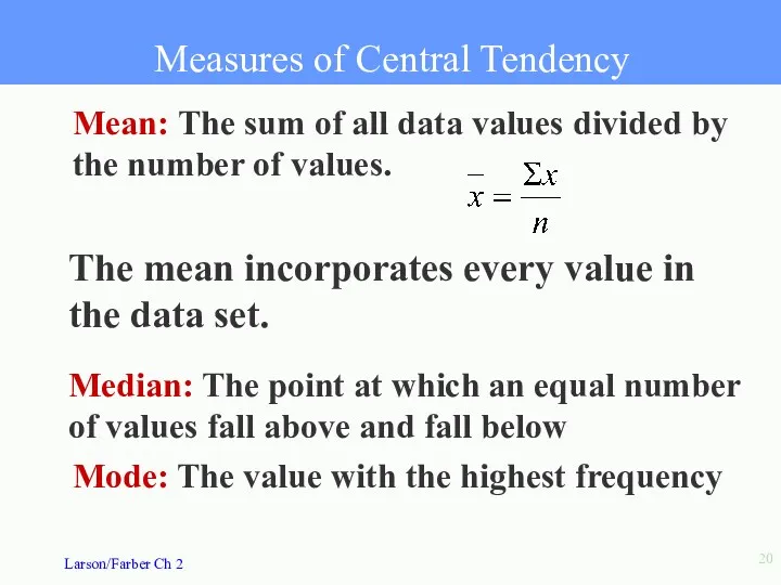
- 20. Measures of Central Tendency Mean: The sum of all data values divided by the number of
- 21. 0 2 2 2 3 4 4 6 40 2 4 2 0 40 2 4
- 22. 2 4 2 0 2 4 3 6 Calculate the mean, the median, and the mode
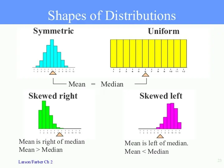
- 23. Uniform Symmetric Skewed right Skewed left Mean is right of median Mean > Median Mean is
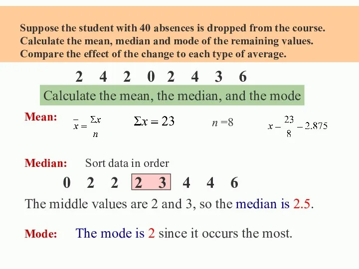
- 24. Outliers What happened to our mean, median and mode when we removed 40 from the data
- 25. Measures of Variation Section 2.4
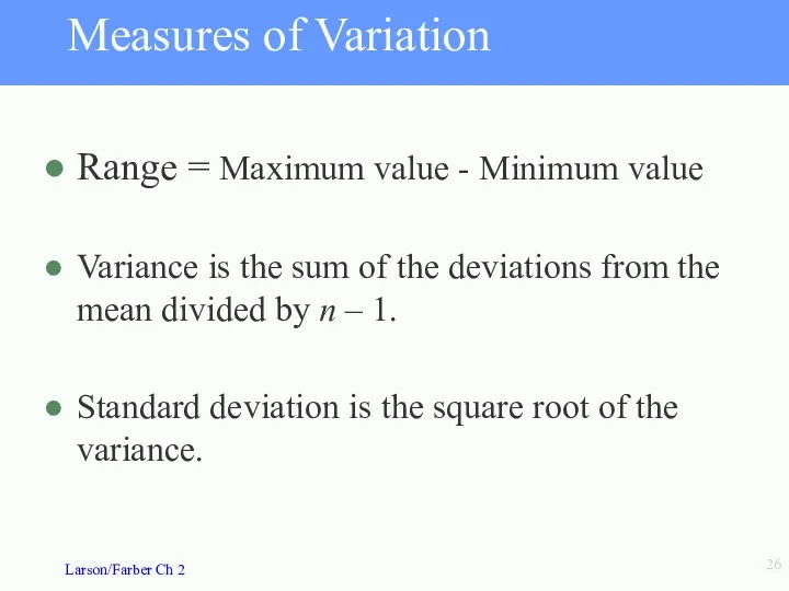
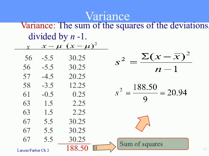
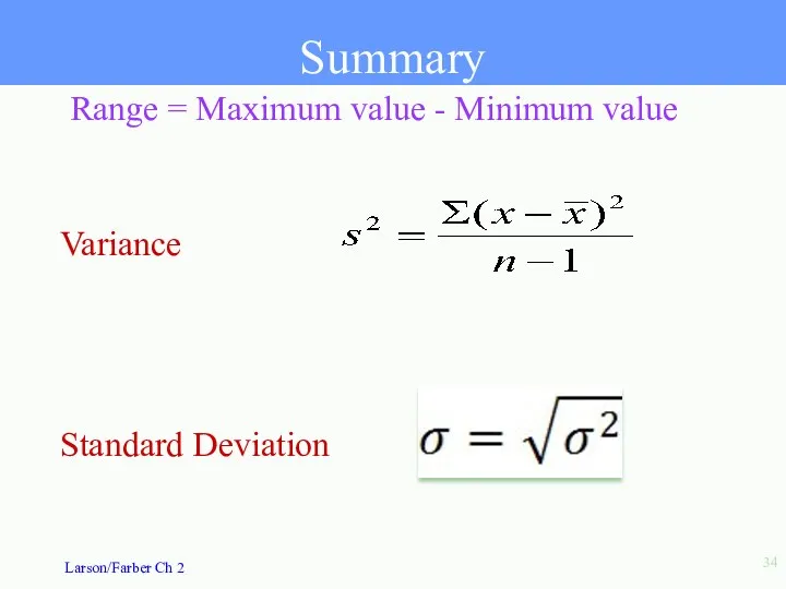
- 26. Measures of Variation Range = Maximum value - Minimum value Variance is the sum of the
- 27. . Example: A testing lab wishes to test two experimental brands of outdoor paint to see
- 28. Closing prices for two stocks were recorded on ten successive Fridays. Calculate the mean, median and
- 29. Range for A = 67 - 56 = $11 Range = Maximum value - Minimum value
- 30. To Calculate Variance & Standard Deviation: 1. Find the deviation, the difference between each data value,
- 31. -5.5 -5.5 -4.5 -3.5 -0.5 1.5 1.5 5.5 5.5 5.5 56 56 57 58 61 63
- 32. Variance: The sum of the squares of the deviations, divided by n -1. x 56 -5.5
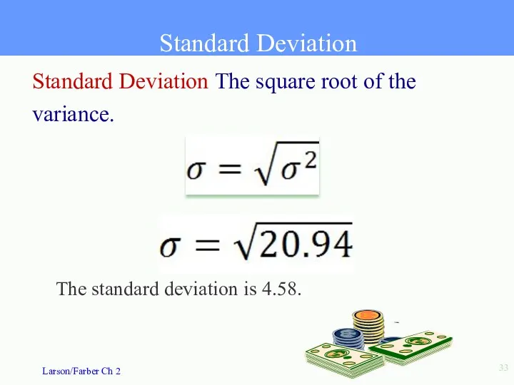
- 33. Standard Deviation Standard Deviation The square root of the variance. The standard deviation is 4.58.
- 34. Summary Standard Deviation Range = Maximum value - Minimum value Variance
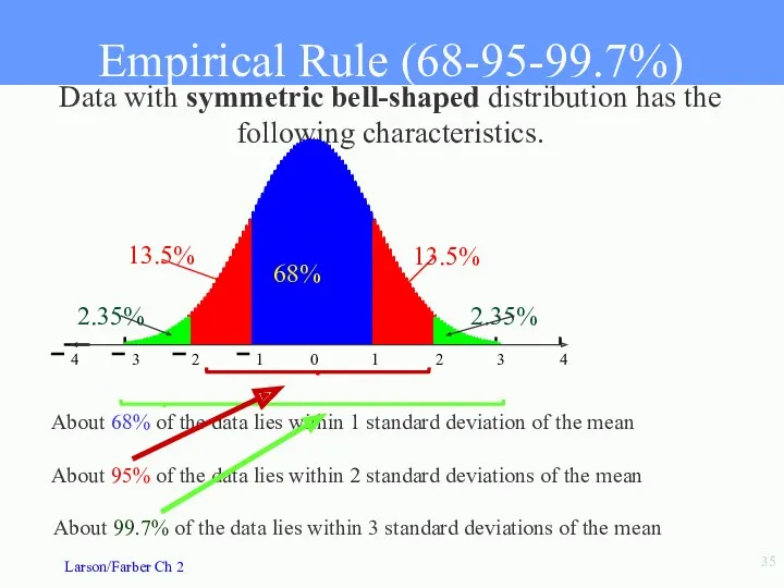
- 35. Data with symmetric bell-shaped distribution has the following characteristics. About 68% of the data lies within
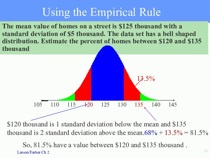
- 36. The mean value of homes on a street is $125 thousand with a standard deviation of
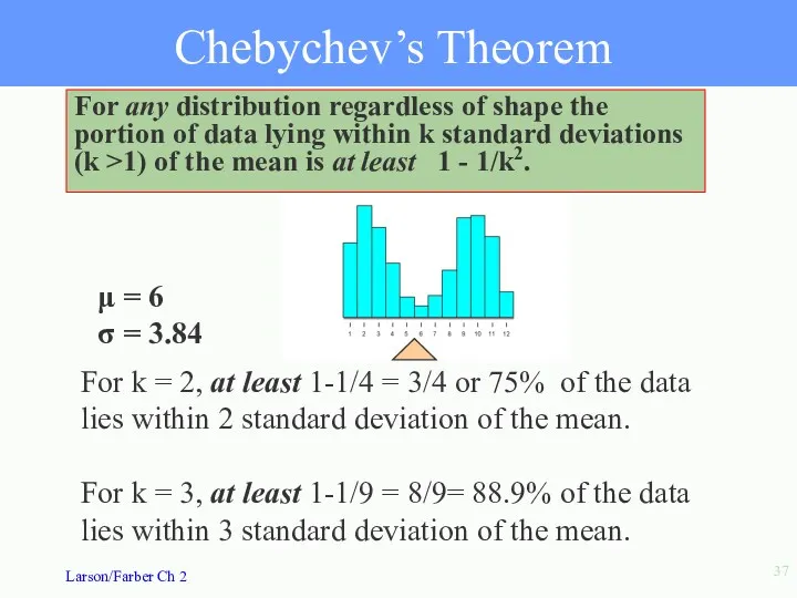
- 37. Chebychev’s Theorem For k = 3, at least 1-1/9 = 8/9= 88.9% of the data lies
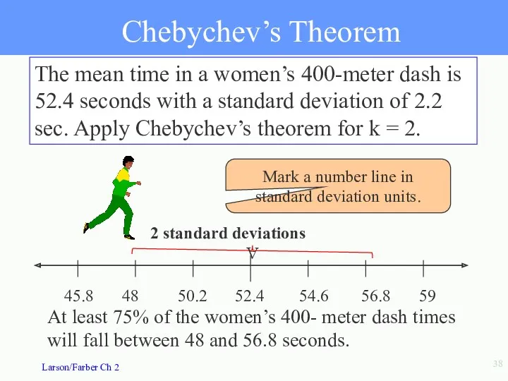
- 38. Chebychev’s Theorem The mean time in a women’s 400-meter dash is 52.4 seconds with a standard
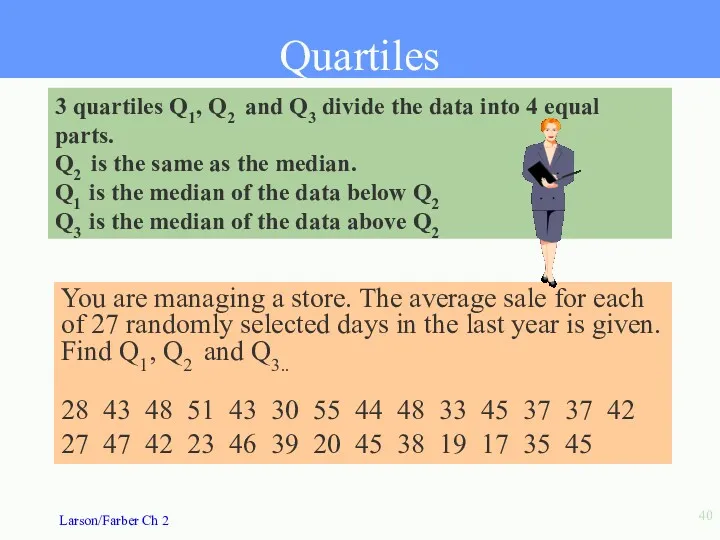
- 39. Measures of Position Section 2.5
- 40. You are managing a store. The average sale for each of 27 randomly selected days in
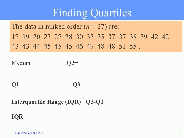
- 41. The data in ranked order (n = 27) are: 17 19 20 23 27 28 30
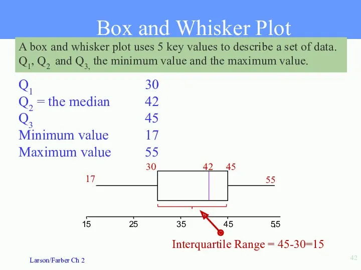
- 42. Box and Whisker Plot A box and whisker plot uses 5 key values to describe a
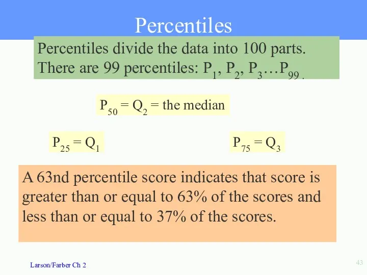
- 43. Percentiles Percentiles divide the data into 100 parts. There are 99 percentiles: P1, P2, P3…P99 .
- 44. Percentiles 114.5 falls on or above 25 of the 30 values. 25/30 = 83.33. So you
- 45. Standard Scores The standard score or z-score, represents the number of standard deviations that a data
- 47. Скачать презентацию
Frequency Distributions and Their Graphs
Section 2.1
Frequency Distributions and Their Graphs
Section 2.1
Frequency Distributions
102 124 108 86 103 82
71 104 112 118 87 95
103 116 85 122 87 100
105
Frequency Distributions
102 124 108 86 103 82
71 104 112 118 87 95
103 116 85 122 87 100
105
4. Mark a tally | in appropriate class for each data
4. Mark a tally | in appropriate class for each data
78
90
102
114
126
3
5
8
9
5
67
79
91
103
115
Do all lower class limits first.
Construct a Frequency
78
90
102
114
126
3
5
8
9
5
67
79
91
103
115
Do all lower class limits first.
Construct a Frequency
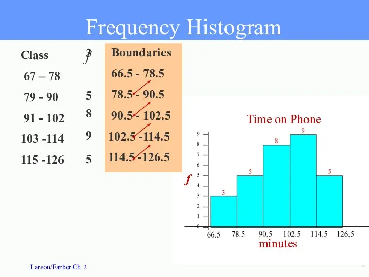
Boundaries
66.5 - 78.5
78.5 - 90.5
90.5 - 102.5
102.5
Boundaries
66.5 - 78.5
78.5 - 90.5
90.5 - 102.5
102.5
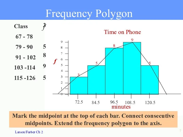
Frequency Polygon
Time on Phone
minutes
f
Mark the midpoint at the top of
Frequency Polygon
Time on Phone
minutes
f
Mark the midpoint at the top of
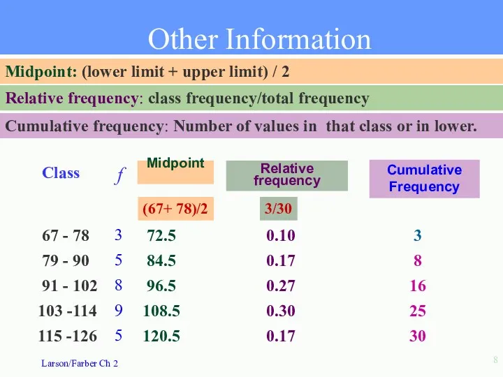
67 - 78
79 - 90
91 - 102
103 -114
115
67 - 78
79 - 90
91 - 102
103 -114
115
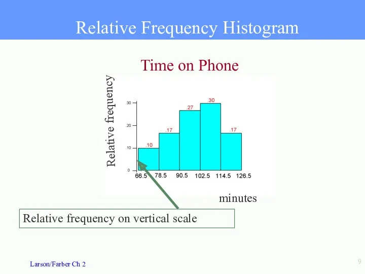
Relative Frequency Histogram
Time on Phone
minutes
Relative frequency
Relative frequency on vertical scale
Relative Frequency Histogram
Time on Phone
minutes
Relative frequency
Relative frequency on vertical scale
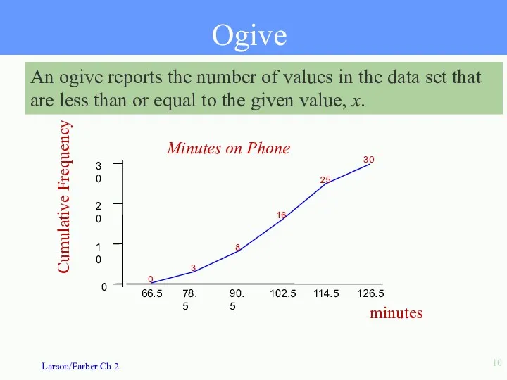
Ogive
An ogive reports the number of values in the data set
Ogive
An ogive reports the number of values in the data set
More Graphs and Displays
Section 2.2
More Graphs and Displays
Section 2.2
Stem-and-Leaf Plot
6 |
7 |
8 |
9 |
10|
11|
12|
Lowest value is 67
Stem-and-Leaf Plot
6 |
7 |
8 |
9 |
10|
11|
12|
Lowest value is 67
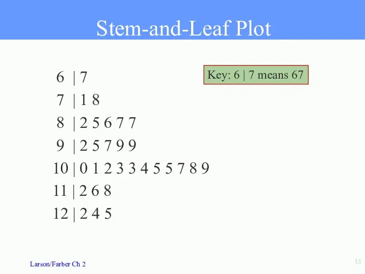
6 | 7
7 | 1 8
8 | 2
6 | 7
7 | 1 8
8 | 2
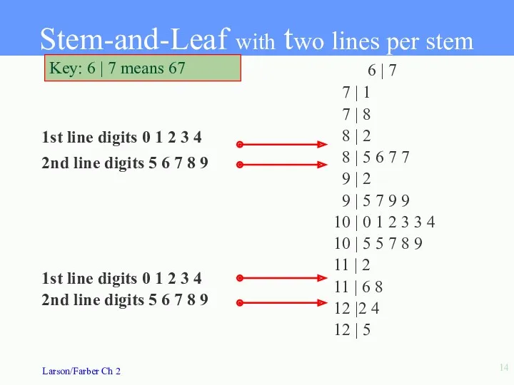
Stem-and-Leaf with two lines per stem
6 | 7
7 |
Stem-and-Leaf with two lines per stem
6 | 7
7 |
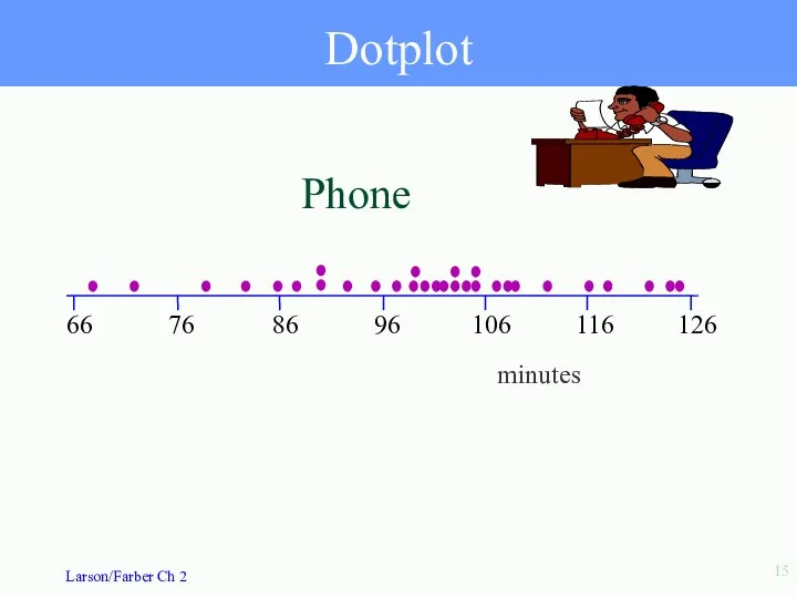
Dotplot
66
76
86
96
106
116
126
Phone
minutes
Dotplot
66
76
86
96
106
116
126
Phone
minutes
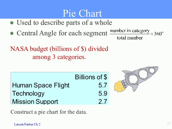
NASA budget (billions of $) divided among 3 categories.
Pie Chart
Used to
NASA budget (billions of $) divided among 3 categories.
Pie Chart
Used to
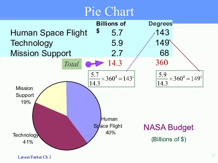
Total
Pie Chart
Billions of $
Human Space Flight
5.7
Technology
5.9
Mission Support
2.7
14.3
Degrees
143
149
68
360
Total
Pie Chart
Billions of $
Human Space Flight
5.7
Technology
5.9
Mission Support
2.7
14.3
Degrees
143
149
68
360
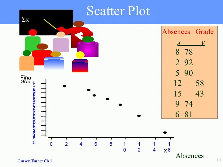
Scatter Plot
x y
8 78
2 92
5 90
12 58
15
Scatter Plot
x y
8 78
2 92
5 90
12 58
15

Measures of Central Tendency
Section 2.3
Measures of Central Tendency
Section 2.3
Measures of Central Tendency
Mean: The sum of all data values divided
Measures of Central Tendency
Mean: The sum of all data values divided
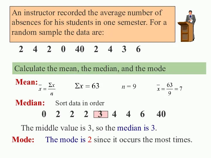
0 2 2 2 3 4 4 6 40
2 4
0 2 2 2 3 4 4 6 40
2 4
2 4 2 0 2 4 3 6
Calculate the mean, the
2 4 2 0 2 4 3 6
Calculate the mean, the
Uniform
Symmetric
Skewed right
Skewed left
Mean is right of median Mean > Median
Mean is
Uniform
Symmetric
Skewed right
Skewed left
Mean is right of median Mean > Median
Mean is
Outliers
What happened to our mean, median and mode when we removed
Outliers
What happened to our mean, median and mode when we removed

Measures of Variation
Section 2.4
Measures of Variation
Section 2.4
Measures of Variation
Range = Maximum value - Minimum value
Variance is the
Measures of Variation
Range = Maximum value - Minimum value
Variance is the
.
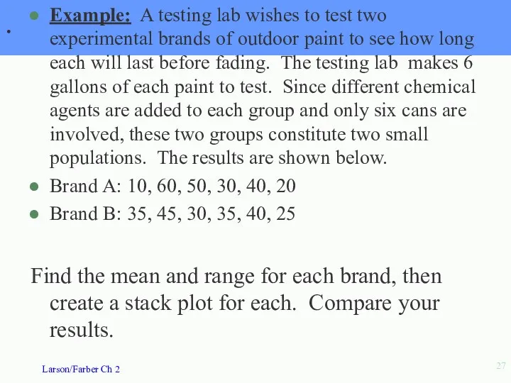
Example: A testing lab wishes to test two experimental brands of
.
Example: A testing lab wishes to test two experimental brands of
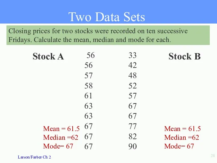
Closing prices for two stocks were recorded on ten successive Fridays.
Closing prices for two stocks were recorded on ten successive Fridays.
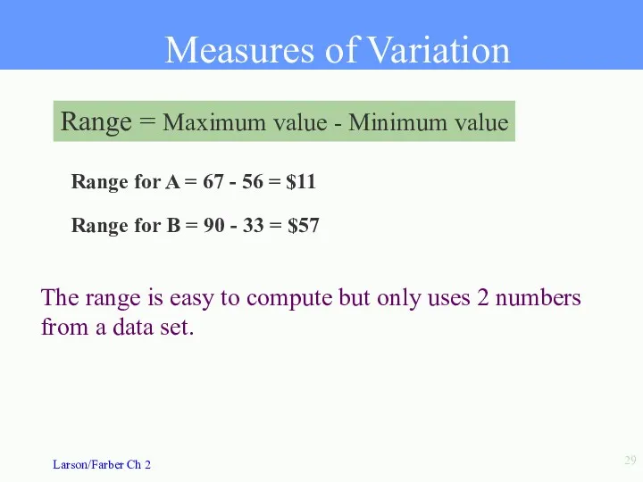
Range for A = 67 - 56 = $11
Range = Maximum
Range for A = 67 - 56 = $11
Range = Maximum
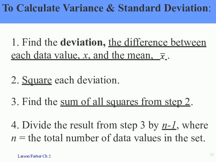
To Calculate Variance & Standard Deviation:
1. Find the deviation, the difference
To Calculate Variance & Standard Deviation:
1. Find the deviation, the difference
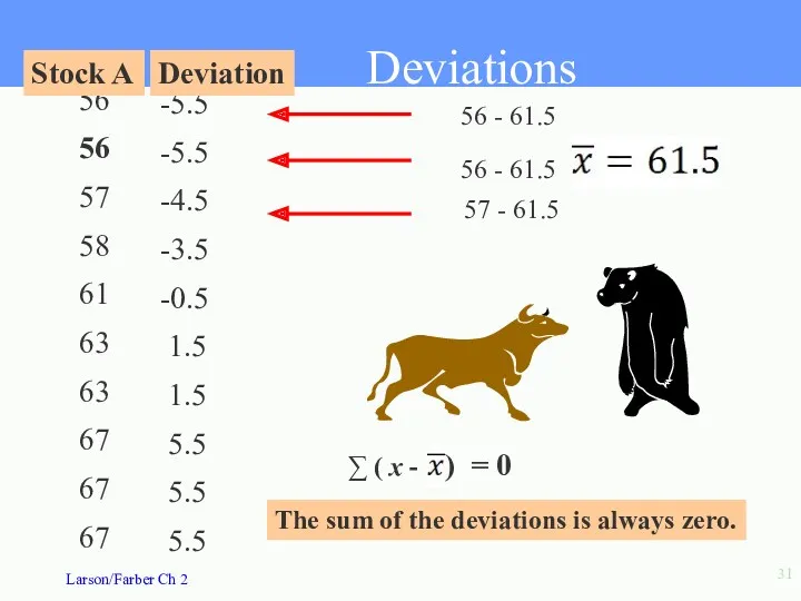
-5.5
-5.5
-4.5
-3.5
-0.5
1.5
-5.5
-5.5
-4.5
-3.5
-0.5
1.5
Variance: The sum of the squares of the deviations, divided by
Variance: The sum of the squares of the deviations, divided by
Standard Deviation
Standard Deviation The square root of the variance.
The standard
Standard Deviation
Standard Deviation The square root of the variance.
The standard
Summary
Standard Deviation
Range = Maximum value - Minimum value
Variance
Summary
Standard Deviation
Range = Maximum value - Minimum value
Variance
Data with symmetric bell-shaped distribution has the following characteristics.
About 68% of
Data with symmetric bell-shaped distribution has the following characteristics.
About 68% of
The mean value of homes on a street is $125 thousand
The mean value of homes on a street is $125 thousand
Chebychev’s Theorem
For k = 3, at least 1-1/9 = 8/9= 88.9%
Chebychev’s Theorem
For k = 3, at least 1-1/9 = 8/9= 88.9%
Chebychev’s Theorem
The mean time in a women’s 400-meter dash is 52.4
Chebychev’s Theorem
The mean time in a women’s 400-meter dash is 52.4
Measures of Position
Section 2.5
Measures of Position
Section 2.5
You are managing a store. The average sale for each of
You are managing a store. The average sale for each of
The data in ranked order (n = 27) are:
17 19 20
The data in ranked order (n = 27) are:
17 19 20
Box and Whisker Plot
A box and whisker plot uses 5 key
Box and Whisker Plot
A box and whisker plot uses 5 key
Percentiles
Percentiles divide the data into 100 parts. There are 99 percentiles:
Percentiles
Percentiles divide the data into 100 parts. There are 99 percentiles:
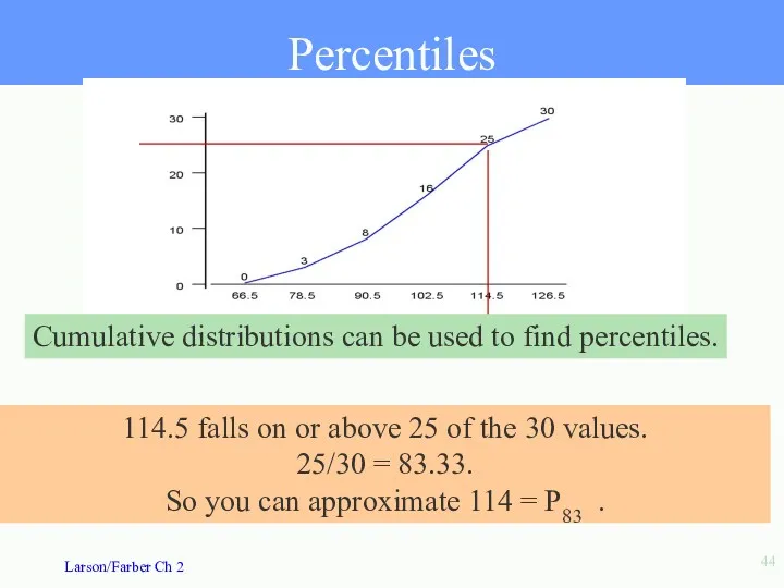
Percentiles
114.5 falls on or above 25 of the 30 values.
25/30
Percentiles
114.5 falls on or above 25 of the 30 values.
25/30
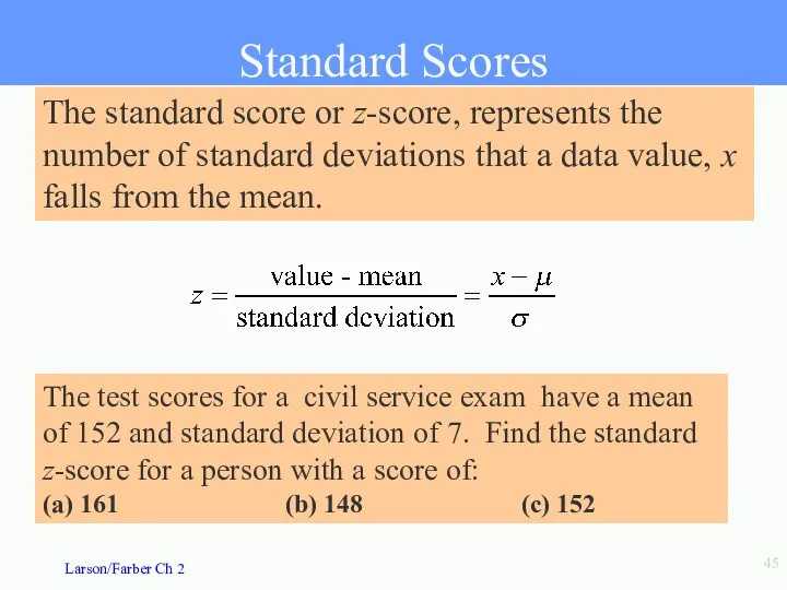
Standard Scores
The standard score or z-score, represents the number of standard
Standard Scores
The standard score or z-score, represents the number of standard
 Відстані в просторі
 Несобственные интегралы. Приложения определённого интеграла. (Лекция 4)
 Открытый урок по математике в 3 классе по теме: Умножение на однозначное число
 Стереометрия (многогранники)
 Умножение обыкновенных дробей. 6 класс
 Веселый счет
 Урок-презентация по математике в 4 классе
 Теория кривых. Кривизна и кручение кривой
 Нахождение площади
 Состав числа
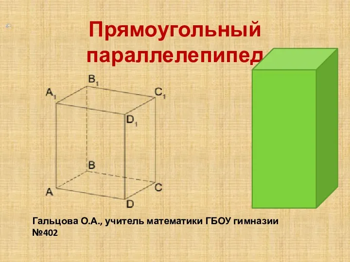 Прямоугольный параллелепипед
 Основы комбинаторики. Перестановки. Размещения
 Килограмм
 Геометрическая интерпретация при решении уравнений, содержащих знак модуля
 Додавання і віднімання числа 6. Урок №45
 Презентация. Задачи по математике 2 класс
 Кривые поверхности
 Математический турнир.
 Урок математики на тему: Круг. Окружность.
 Лекция 01. Теория вероятностей
 Функциональные и степенные ряды
 Что такое положительное и что такое отрицательное число?
 Презентация - конспект НОД Дорога к солнышку
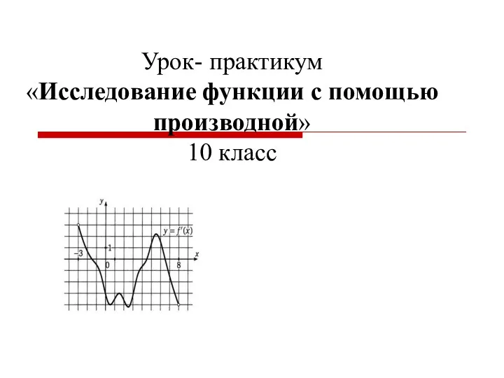 Урок- практикум Исследование функции с помощью производной 10 класс
 Формирование интереса к математике у детей старшего дошкольного возраста
 Деление дробей. Обобщение. 6 класс
 Лабораторная № 6. Численное решение систем линейных алгебраических уравнений
 Модуль числа (6 класс)