- Introduction to normal distributions

Содержание
- 2. Section 6-1 Objectives Interpret graphs of normal probability distributions Find areas under the standard normal curve
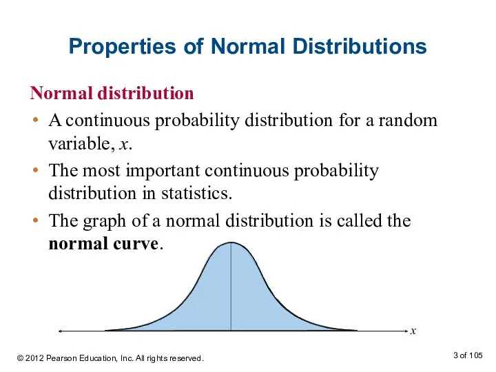
- 3. Properties of Normal Distributions Normal distribution A continuous probability distribution for a random variable, x. The
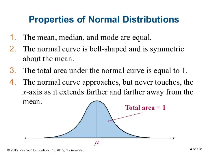
- 4. Properties of Normal Distributions The mean, median, and mode are equal. The normal curve is bell-shaped
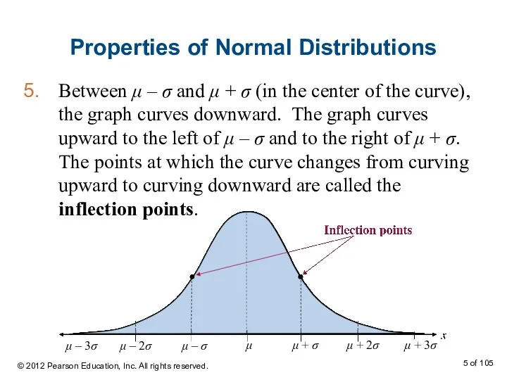
- 5. Properties of Normal Distributions Between μ – σ and μ + σ (in the center of
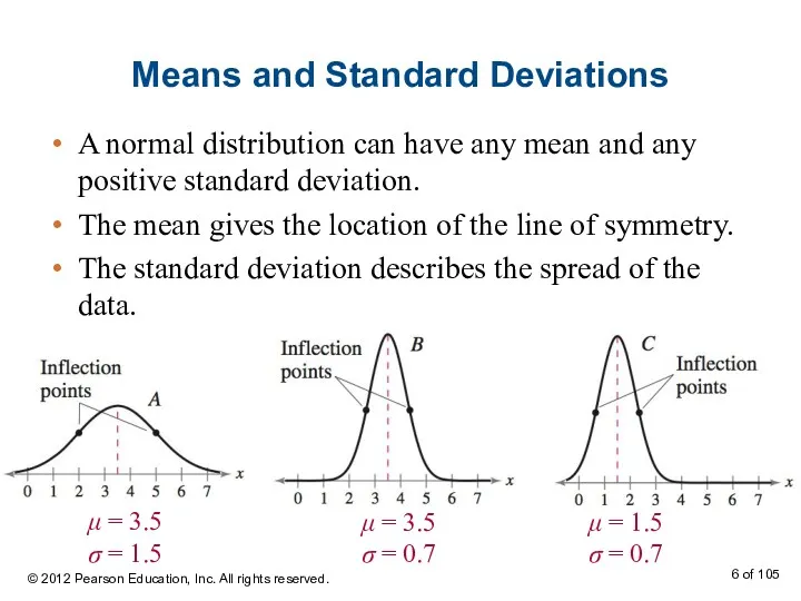
- 6. Means and Standard Deviations A normal distribution can have any mean and any positive standard deviation.
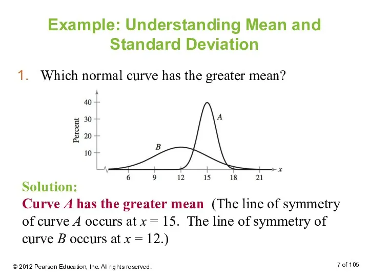
- 7. Example: Understanding Mean and Standard Deviation Which normal curve has the greater mean? Solution: Curve A
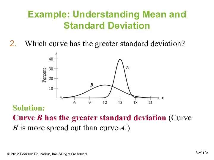
- 8. Example: Understanding Mean and Standard Deviation Which curve has the greater standard deviation? Solution: Curve B
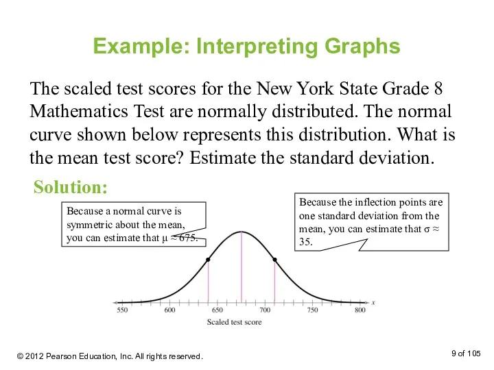
- 9. Example: Interpreting Graphs The scaled test scores for the New York State Grade 8 Mathematics Test
- 10. The Standard Normal Distribution Standard normal distribution A normal distribution with a mean of 0 and
- 11. The Standard Normal Distribution If each data value of a normally distributed random variable x is
- 12. Properties of the Standard Normal Distribution The cumulative area is close to 0 for z-scores close
- 13. Properties of the Standard Normal Distribution The cumulative area for z = 0 is 0.5000. The
- 14. Example: Using The Standard Normal Table Find the cumulative area that corresponds to a z-score of
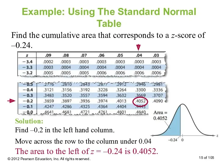
- 15. Example: Using The Standard Normal Table Find the cumulative area that corresponds to a z-score of
- 16. Finding Areas Under the Standard Normal Curve Sketch the standard normal curve and shade the appropriate
- 17. Finding Areas Under the Standard Normal Curve To find the area to the right of z,
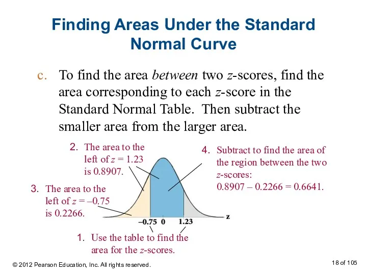
- 18. Finding Areas Under the Standard Normal Curve To find the area between two z-scores, find the
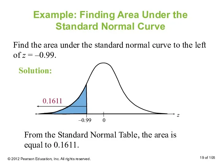
- 19. Example: Finding Area Under the Standard Normal Curve Find the area under the standard normal curve
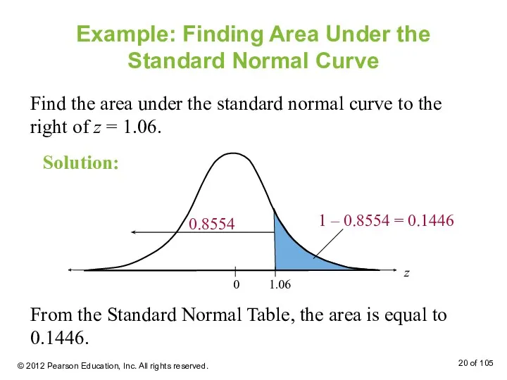
- 20. Example: Finding Area Under the Standard Normal Curve Find the area under the standard normal curve
- 22. Скачать презентацию
Section 6-1 Objectives
Interpret graphs of normal probability distributions
Find areas under the
Section 6-1 Objectives
Interpret graphs of normal probability distributions
Find areas under the
Properties of Normal Distributions
Normal distribution
A continuous probability distribution for a
Properties of Normal Distributions
Normal distribution
A continuous probability distribution for a
Properties of Normal Distributions
The mean, median, and mode are equal.
The normal
Properties of Normal Distributions
The mean, median, and mode are equal.
The normal
Properties of Normal Distributions
Between μ – σ and μ + σ
Properties of Normal Distributions
Between μ – σ and μ + σ
Means and Standard Deviations
A normal distribution can have any mean and
Means and Standard Deviations
A normal distribution can have any mean and
Example: Understanding Mean and Standard Deviation
Which normal curve has the greater
Example: Understanding Mean and Standard Deviation
Which normal curve has the greater
Example: Understanding Mean and Standard Deviation
Which curve has the greater standard
Example: Understanding Mean and Standard Deviation
Which curve has the greater standard
Example: Interpreting Graphs
The scaled test scores for the New York State
Example: Interpreting Graphs
The scaled test scores for the New York State
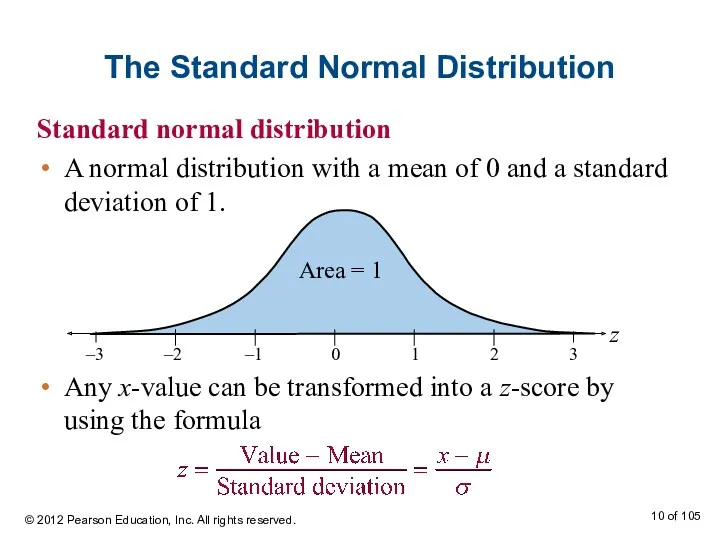
The Standard Normal Distribution
Standard normal distribution
A normal distribution with a
The Standard Normal Distribution
Standard normal distribution
A normal distribution with a
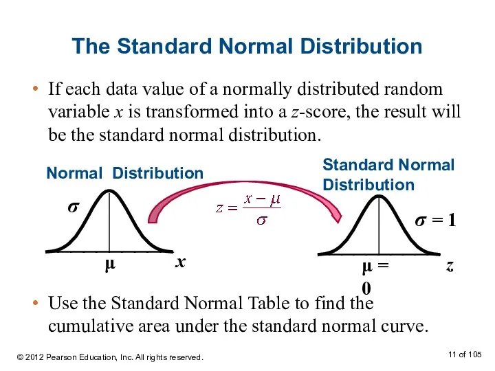
The Standard Normal Distribution
If each data value of a normally distributed
The Standard Normal Distribution
If each data value of a normally distributed
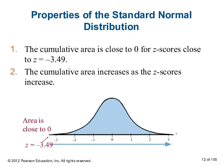
Properties of the Standard Normal Distribution
The cumulative area is close to
Properties of the Standard Normal Distribution
The cumulative area is close to
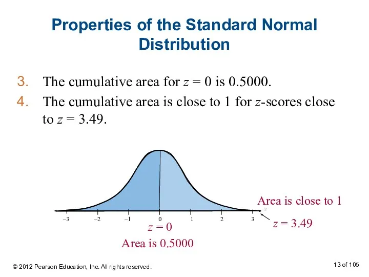
Properties of the Standard Normal Distribution
The cumulative area for z =
Properties of the Standard Normal Distribution
The cumulative area for z =
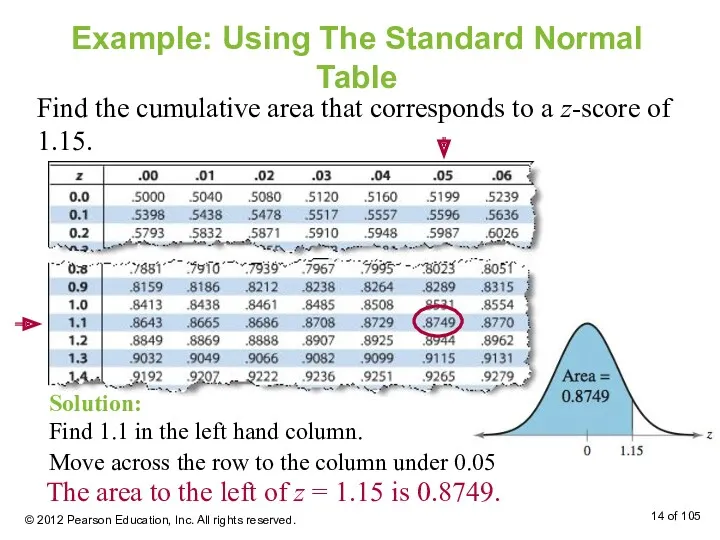
Example: Using The Standard Normal Table
Find the cumulative area that corresponds
Example: Using The Standard Normal Table
Find the cumulative area that corresponds
Example: Using The Standard Normal Table
Find the cumulative area that corresponds
Example: Using The Standard Normal Table
Find the cumulative area that corresponds
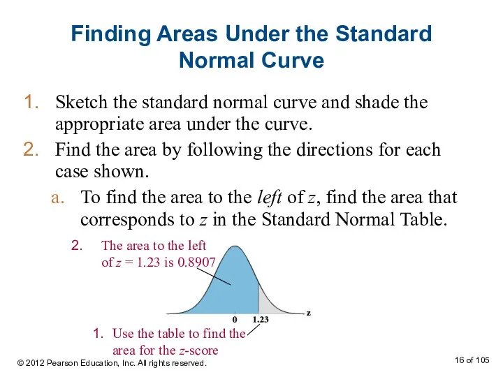
Finding Areas Under the Standard Normal Curve
Sketch the standard normal curve
Finding Areas Under the Standard Normal Curve
Sketch the standard normal curve
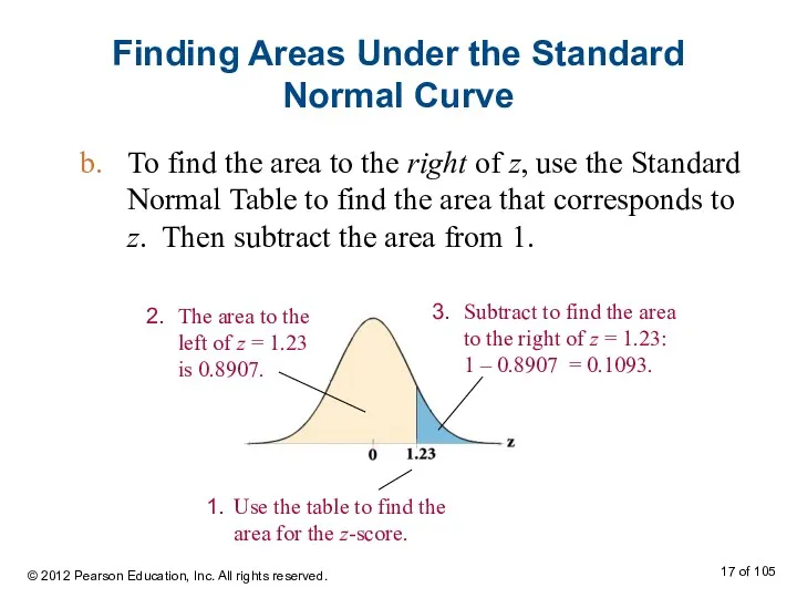
Finding Areas Under the Standard Normal Curve
To find the area to
Finding Areas Under the Standard Normal Curve
To find the area to
Finding Areas Under the Standard Normal Curve
To find the area between
Finding Areas Under the Standard Normal Curve
To find the area between
Example: Finding Area Under the Standard Normal Curve
Find the area under
Example: Finding Area Under the Standard Normal Curve
Find the area under
Example: Finding Area Under the Standard Normal Curve
Find the area under
Example: Finding Area Under the Standard Normal Curve
Find the area under
 Марковские цепи
 Умножение трёхзначного числа на однозначное
 Использование координат и векторов при решении прикладных задач
 Золотое сечение
 Правильные и неправильные дроби. Понятия
 Производная в химии
 Презентация Волшебный мир геометрических фигур
 Статистические показатели
 Десятичная система счисления. Римские цифры
 Тренажёр. Умножение и деление на 5
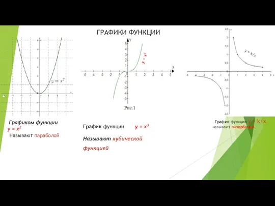 Графики функции. Кубическая парабола
 Divide et impera. Metodei şi aplicaţii
 Дәрес планы
 Двугранный угол. Признак перпендикулярности двух плоскостей
 Презентация к уроку математики Прямой и обратный порядок Диск
 Открытый урок математики во 2 классе. Тема Вычитание суммы из числа
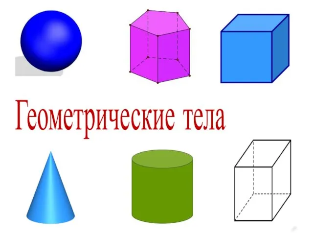 Геометрические тела
 Решение треугольников
 Определение угла. Развернутый угол. Сравнение углов наложением
 Числовые выражения
 Знакомство с архитектоникой здания
 Деление дробей. 8 класс
 Сложная функция. Производная сложной функции
 Әй, осы математика
 Применение методов статистического анализа для изучения общественного здоровья
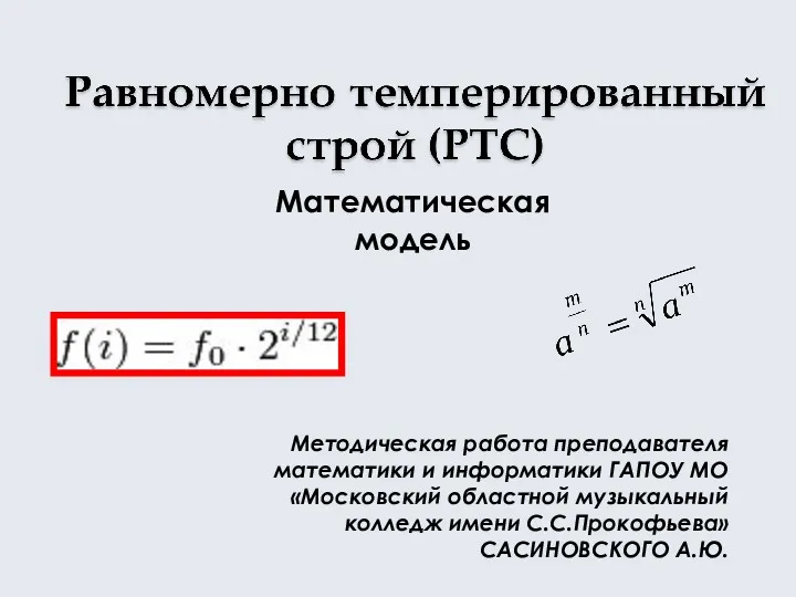 Равномерно темперированный строй. Математиечская модель
 Независимые повторные испытания
 Таблица вариантов и правило произведения