- Lemke’s Algorithm: The Hammer in Your Math Toolbox?

Содержание
- 2. First, a Word About Hammers requirements for this to be a good idea a way of
- 3. Hammers (cont.) by definition, not the optimal way to solve problems, BUT computers are very fast
- 4. What are “advanced game math problems”? problems that are ammenable to mathematical modeling state the problem
- 5. Prerequisites linear algebra vector, matrix symbol manipulation at least calculus concepts what derivatives mean comfortable with
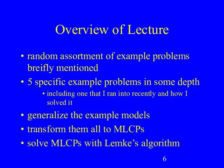
- 6. Overview of Lecture random assortment of example problems breifly mentioned 5 specific example problems in some
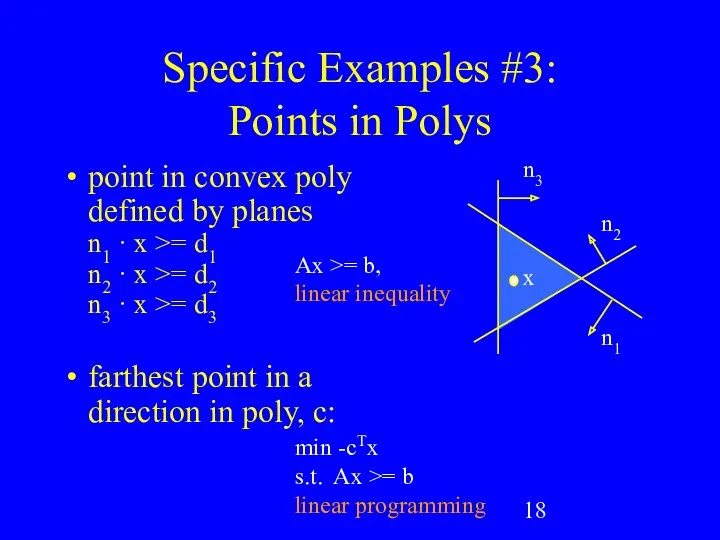
- 7. A Look Forward linear equations Ax = b linear inequalities Ax >= b linear programming min
- 8. Applications to Games graphics, physics, ai, even ui computational geometry visibility contact curve fitting constraints integration
- 9. Applications to Games (cont.) don’t forget... The Elastohydrodynamic Lubrication Problem Solving Optimal Ownership Structures “The two
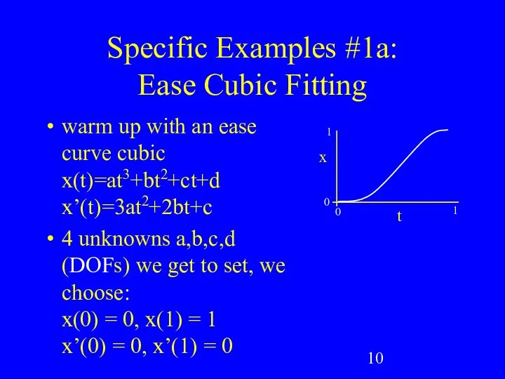
- 10. Specific Examples #1a: Ease Cubic Fitting warm up with an ease curve cubic x(t)=at3+bt2+ct+d x’(t)=3at2+2bt+c 4
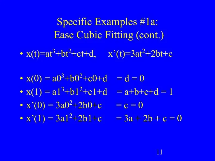
- 11. Specific Examples #1a: Ease Cubic Fitting (cont.) x(t)=at3+bt2+ct+d, x’(t)=3at2+2bt+c x(0) = a03+b02+c0+d = d = 0
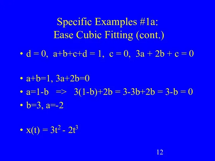
- 12. Specific Examples #1a: Ease Cubic Fitting (cont.) d = 0, a+b+c+d = 1, c = 0,
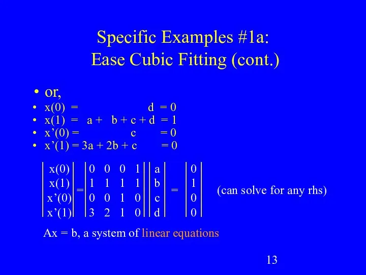
- 13. Specific Examples #1a: Ease Cubic Fitting (cont.) or, x(0) = d = 0 x(1) = a
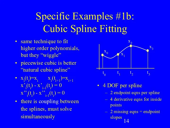
- 14. Specific Examples #1b: Cubic Spline Fitting same technique to fit higher order polynomials, but they “wiggle”
- 15. Specific Examples #1b: Cubic Spline Fitting (cont.) a0 b0 c0 d0 a1 b1 c1 d1 .
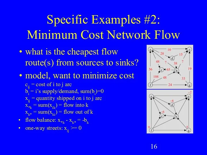
- 16. Specific Examples #2: Minimum Cost Network Flow what is the cheapest flow route(s) from sources to
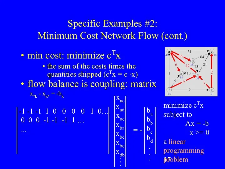
- 17. Specific Examples #2: Minimum Cost Network Flow (cont.) min cost: minimize cTx the sum of the
- 18. Specific Examples #3: Points in Polys point in convex poly defined by planes n1 · x
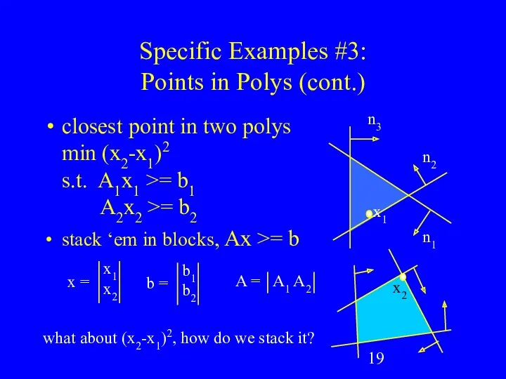
- 19. Specific Examples #3: Points in Polys (cont.) closest point in two polys min (x2-x1)2 s.t. A1x1
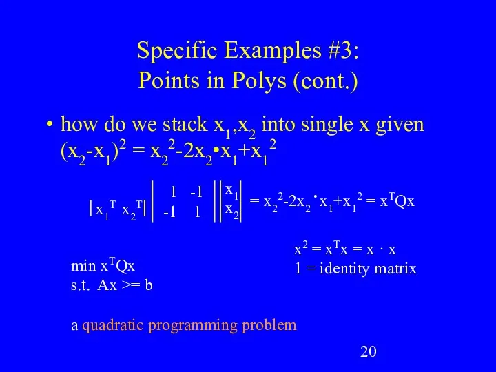
- 20. Specific Examples #3: Points in Polys (cont.) how do we stack x1,x2 into single x given
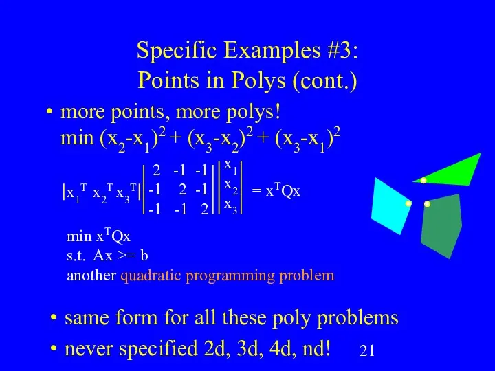
- 21. Specific Examples #3: Points in Polys (cont.) more points, more polys! min (x2-x1)2 + (x3-x2)2 +
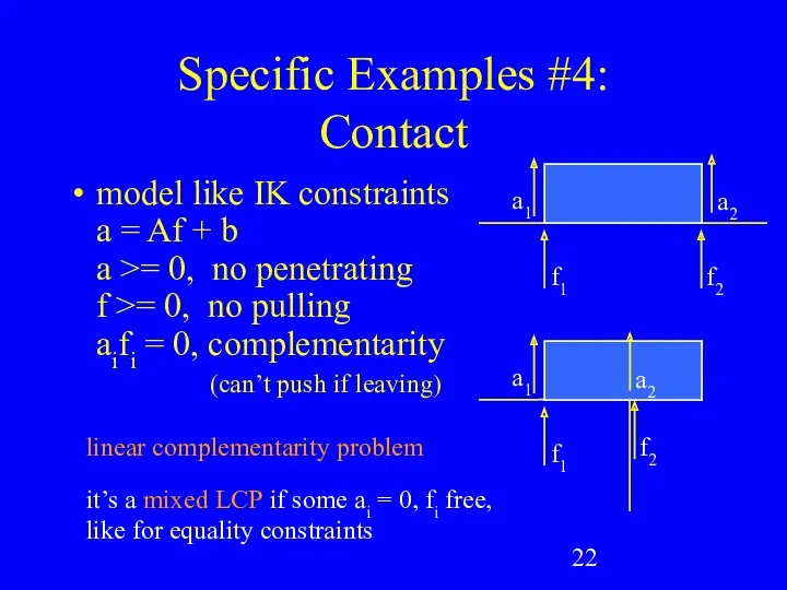
- 22. Specific Examples #4: Contact model like IK constraints a = Af + b a >= 0,
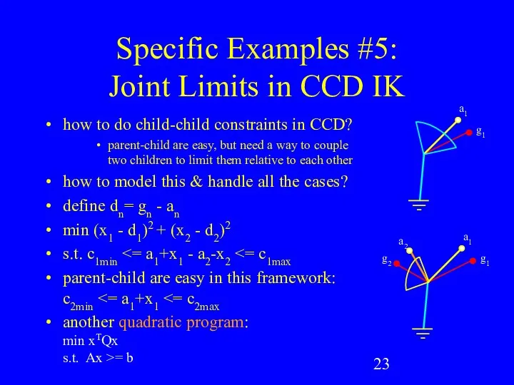
- 23. Specific Examples #5: Joint Limits in CCD IK how to do child-child constraints in CCD? parent-child
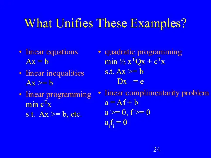
- 24. What Unifies These Examples? linear equations Ax = b linear inequalities Ax >= b linear programming
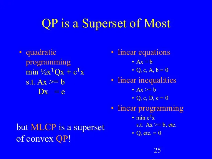
- 25. QP is a Superset of Most quadratic programming min ½xTQx + cTx s.t. Ax >= b
- 26. Karush-Kuhn-Tucker Optimality Conditions get us to MLCP for QP form “Lagrangian” L(x,u,v) = ½ xTQx +
- 27. Karush-Kuhn-Tucker Optimality Conditions (cont.) L(x,u,v) = ½ xTQx + cTx - uT(Ax - b) - vT(Dx
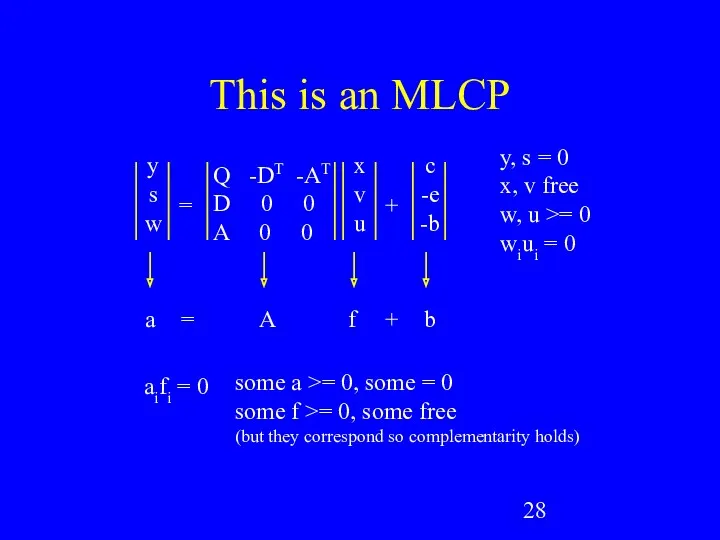
- 28. This is an MLCP x v u Q -DT -AT D 0 0 A 0 0
- 29. Modeling Summary a lot of interesting problems can be formulated as MLCPs model the problem mathematically
- 30. Solving MLCPs (where I hope I made you hungry enough for homework) Lemke’s Algorithm is only
- 31. Playing Around With MLCPs PATH, a MCP solver (superset of MLCP!) really stoked professional solver free
- 32. References for Lemke, etc. free pdf book by Katta Murty on LCPs, etc. free pdf book
- 34. Specific Examples #5: Constraints for IK compute “forces” to keep bones together a1 = A11 f1
- 36. Скачать презентацию
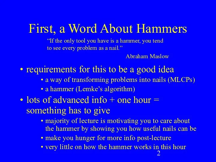
First, a Word About Hammers
requirements for this to be a good
First, a Word About Hammers
requirements for this to be a good
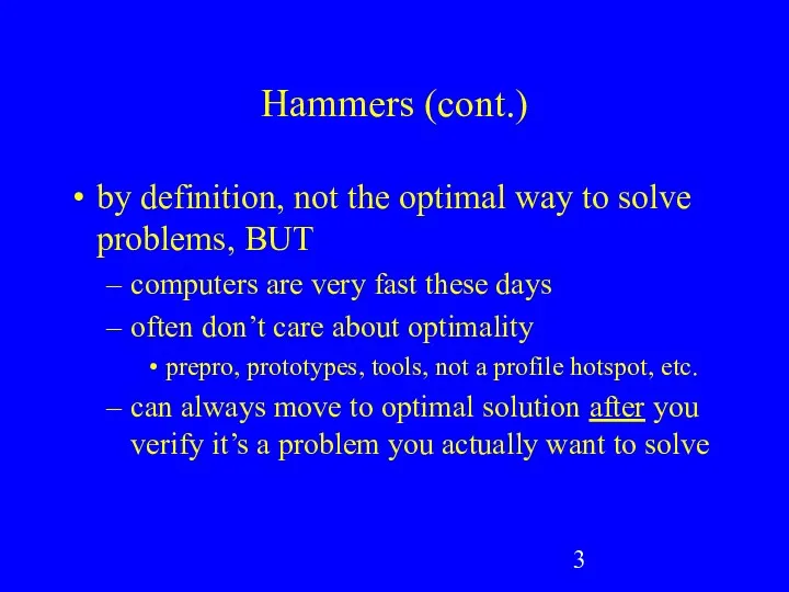
Hammers (cont.)
by definition, not the optimal way to solve problems, BUT
computers
Hammers (cont.)
by definition, not the optimal way to solve problems, BUT
computers
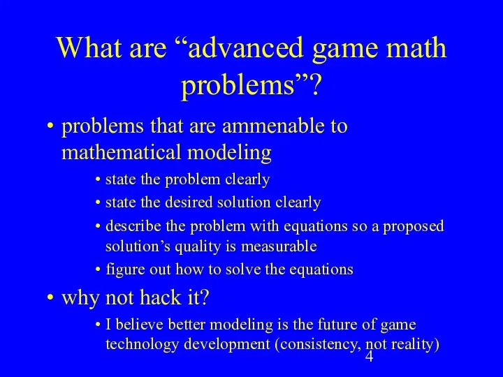
What are “advanced game math problems”?
problems that are ammenable to mathematical
What are “advanced game math problems”?
problems that are ammenable to mathematical
Prerequisites
linear algebra
vector, matrix symbol manipulation at least
calculus concepts
what derivatives mean
comfortable with
Prerequisites
linear algebra
vector, matrix symbol manipulation at least
calculus concepts
what derivatives mean
comfortable with
Overview of Lecture
random assortment of example problems breifly mentioned
5 specific example
Overview of Lecture
random assortment of example problems breifly mentioned
5 specific example
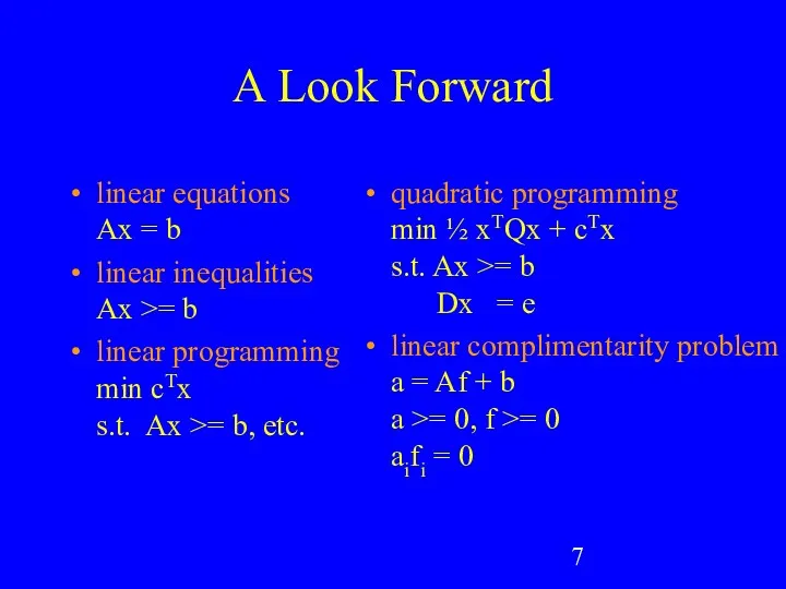
A Look Forward
linear equations
Ax = b
linear inequalities
Ax >= b
linear programming
min
A Look Forward
linear equations
Ax = b
linear inequalities
Ax >= b
linear programming
min
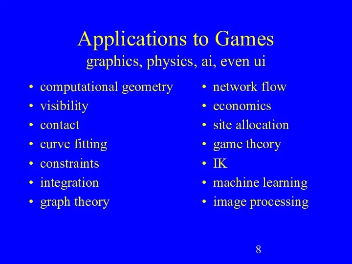
Applications to Games
graphics, physics, ai, even ui
computational geometry
visibility
contact
curve fitting
constraints
integration
graph theory
network flow
economics
site
Applications to Games
graphics, physics, ai, even ui
computational geometry
visibility
contact
curve fitting
constraints
integration
graph theory
network flow
economics
site
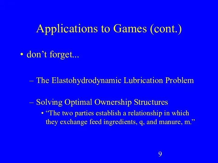
Applications to Games (cont.)
don’t forget...
The Elastohydrodynamic Lubrication Problem
Solving Optimal Ownership Structures
“The
Applications to Games (cont.)
don’t forget...
The Elastohydrodynamic Lubrication Problem
Solving Optimal Ownership Structures
“The
Specific Examples #1a:
Ease Cubic Fitting
warm up with an ease curve
Specific Examples #1a:
Ease Cubic Fitting
warm up with an ease curve
Specific Examples #1a: Ease Cubic Fitting (cont.)
x(t)=at3+bt2+ct+d, x’(t)=3at2+2bt+c
x(0) = a03+b02+c0+d =
Specific Examples #1a: Ease Cubic Fitting (cont.)
x(t)=at3+bt2+ct+d, x’(t)=3at2+2bt+c
x(0) = a03+b02+c0+d =
Specific Examples #1a: Ease Cubic Fitting (cont.)
d = 0, a+b+c+d =
Specific Examples #1a: Ease Cubic Fitting (cont.)
d = 0, a+b+c+d =
Specific Examples #1a: Ease Cubic Fitting (cont.)
or,
x(0) = d = 0
x(1)
Specific Examples #1a: Ease Cubic Fitting (cont.)
or,
x(0) = d = 0
x(1)
Specific Examples #1b:
Cubic Spline Fitting
same technique to fit higher order
Specific Examples #1b:
Cubic Spline Fitting
same technique to fit higher order
Specific Examples #1b:
Cubic Spline Fitting (cont.)
a0
b0
c0
d0
a1
b1
c1
d1
.
.
.
x0
x1
0
0
x1
x2
0
0
.
.
.
=
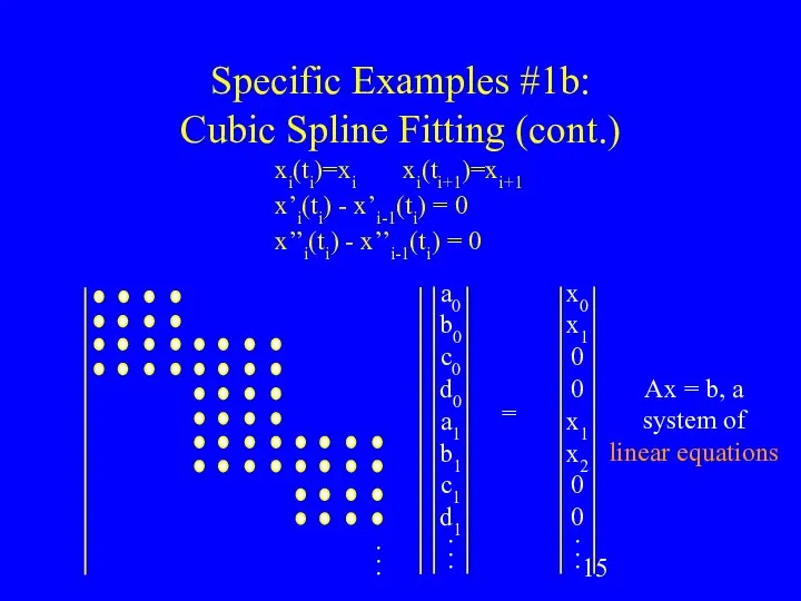
xi(ti)=xi xi(ti+1)=xi+1
x’i(ti) - x’i-1(ti) =
Specific Examples #1b:
Cubic Spline Fitting (cont.)
a0
b0
c0
d0
a1
b1
c1
d1
.
.
.
x0
x1
0
0
x1
x2
0
0
.
.
.
=
xi(ti)=xi xi(ti+1)=xi+1 x’i(ti) - x’i-1(ti) =
Specific Examples #2:
Minimum Cost Network Flow
what is the cheapest flow
Specific Examples #2:
Minimum Cost Network Flow
what is the cheapest flow
Specific Examples #2:
Minimum Cost Network Flow (cont.)
min cost: minimize cTx
the
Specific Examples #2:
Minimum Cost Network Flow (cont.)
min cost: minimize cTx
the
Specific Examples #3:
Points in Polys
point in convex poly defined by
Specific Examples #3:
Points in Polys
point in convex poly defined by
Specific Examples #3:
Points in Polys (cont.)
closest point in two polys
min
Specific Examples #3:
Points in Polys (cont.)
closest point in two polys min
Specific Examples #3:
Points in Polys (cont.)
how do we stack x1,x2
Specific Examples #3:
Points in Polys (cont.)
how do we stack x1,x2
Specific Examples #3:
Points in Polys (cont.)
more points, more polys!
min (x2-x1)2
Specific Examples #3:
Points in Polys (cont.)
more points, more polys! min (x2-x1)2
Specific Examples #4:
Contact
model like IK constraints
a = Af + b
a
Specific Examples #4:
Contact
model like IK constraints a = Af + b a
Specific Examples #5:
Joint Limits in CCD IK
how to do child-child
Specific Examples #5:
Joint Limits in CCD IK
how to do child-child
What Unifies These Examples?
linear equations
Ax = b
linear inequalities
Ax >= b
linear
What Unifies These Examples?
linear equations
Ax = b
linear inequalities
Ax >= b
linear
QP is a Superset of Most
quadratic programming
min ½xTQx + cTx
s.t. Ax
QP is a Superset of Most
quadratic programming min ½xTQx + cTx s.t. Ax
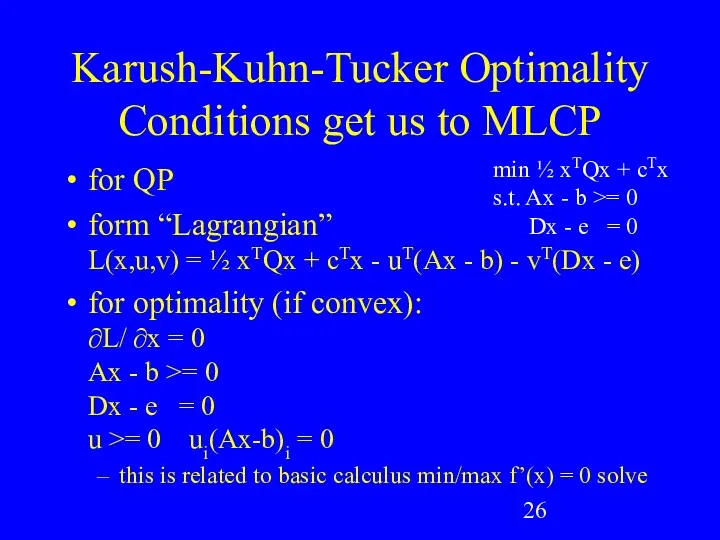
Karush-Kuhn-Tucker Optimality Conditions get us to MLCP
for QP
form “Lagrangian”
L(x,u,v) = ½
Karush-Kuhn-Tucker Optimality Conditions get us to MLCP
for QP
form “Lagrangian”
L(x,u,v) = ½
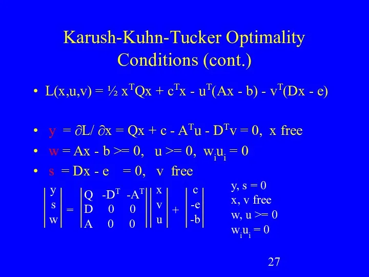
Karush-Kuhn-Tucker Optimality Conditions (cont.)
L(x,u,v) = ½ xTQx + cTx - uT(Ax
Karush-Kuhn-Tucker Optimality Conditions (cont.)
L(x,u,v) = ½ xTQx + cTx - uT(Ax
This is an MLCP
x
v
u
Q -DT -AT
D 0 0
A 0 0
=
y
s
w
+
c
-e
-b
y, s
This is an MLCP
x
v
u
Q -DT -AT
D 0 0
A 0 0
=
y
s
w
+
c
-e
-b
y, s
Modeling Summary
a lot of interesting problems can be formulated as MLCPs
model
Modeling Summary
a lot of interesting problems can be formulated as MLCPs
model
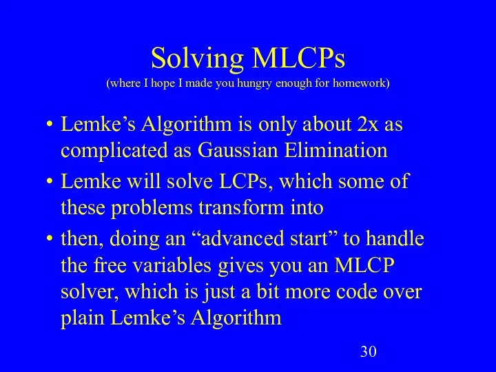
Solving MLCPs
(where I hope I made you hungry enough for homework)
Lemke’s
Solving MLCPs
(where I hope I made you hungry enough for homework)
Lemke’s
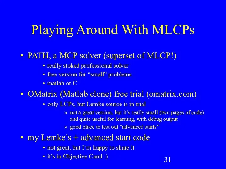
Playing Around With MLCPs
PATH, a MCP solver (superset of MLCP!)
really stoked
Playing Around With MLCPs
PATH, a MCP solver (superset of MLCP!)
really stoked
References for Lemke, etc.
free pdf book by Katta Murty on LCPs,
References for Lemke, etc.
free pdf book by Katta Murty on LCPs,

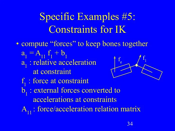
Specific Examples #5:
Constraints for IK
compute “forces” to keep bones together
a1
Specific Examples #5:
Constraints for IK
compute “forces” to keep bones together a1
 Треугольники. Задачи
 Метод координат при решении стереометрических задач. Урок геометрии, 11 класс
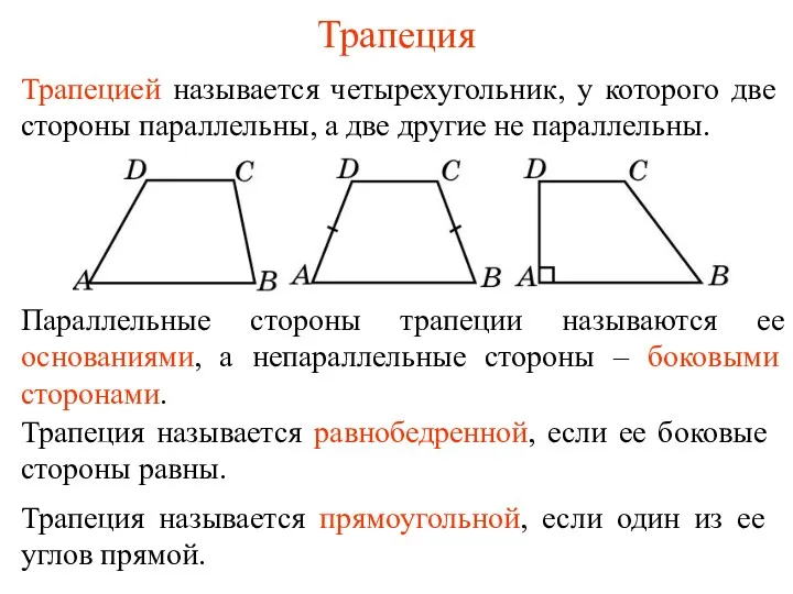 Трапеция. Теорема о средней линии трапеции
 Признаки делимости чисел на 2, 3, 9
 Конус. Элементы конуса. Сечение конуса
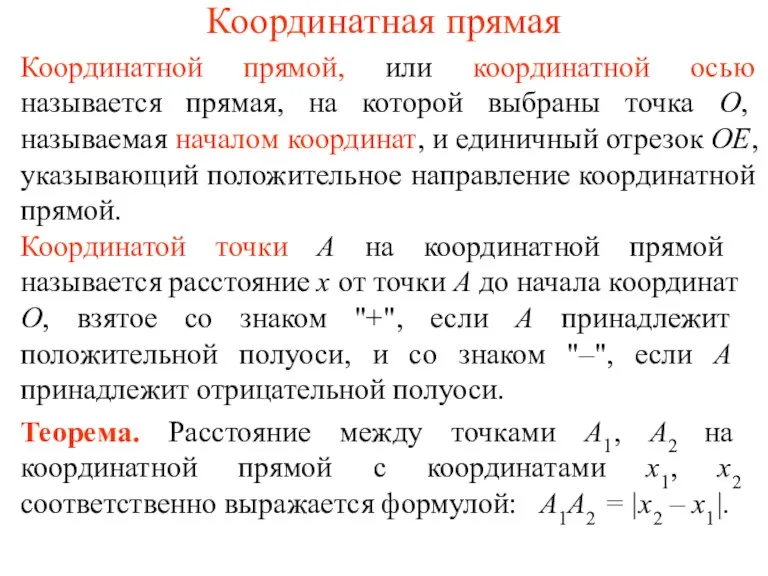 Координатная прямая
 Сложная функция. 10 класс
 презентации и конспекты уроков
 Прогрессии вокруг нас. (9 класс)
 Число и цифра 4
 Презентация по математике тема: Часы, минуты, сутки (подготовительная группа)
 Корреляционно-регрессионный анализ
 Измерение углов
 Цилиндр
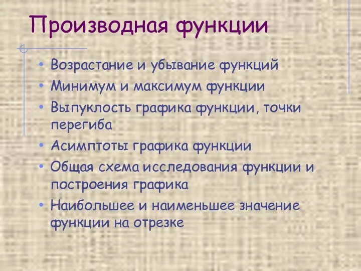 Производная функции. Возрастание и убывание функций
 Интеллектуальная математическая игра для 6 класса
 Сложение и вычитание в пределах 20 2 класс УМК Школа 2100
 Урок математики Движение с отставанием 4 класс Петерсон Л. Г.
 Численные методы
 Признаки параллельности прямых
 Квадратный корень. Арифметический квадратный корень
 Розкладання квадратного тричлена на множники
 Площадь фигуры
 Плоские фигуры - многоугольники. Объемные фигуры
 Функция. Область определения и область значений функции. 7 класс
 Презентация к уроку математики Зимние забавы
 Линейная модель парной регрессии. Метод наименьших квадратов
 Начальные геометрические сведения. Прямая и отрезок