- Linear Regression. Linear Regression with Gradient Descent. Regularization. Lecture 4.2

Содержание
- 2. Lecture 4.2 Linear Regression. Linear Regression with Gradient Descent. Regularization
- 3. https://www.youtube.com/watch?v=vMh0zPT0tLI https://www.youtube.com/watch?v=Q81RR3yKn30 https://www.youtube.com/watch?v=NGf0voTMlcs https://www.youtube.com/watch?v=1dKRdX9bfIo
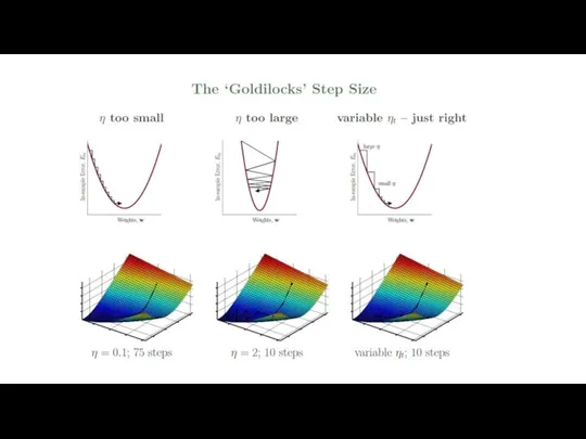
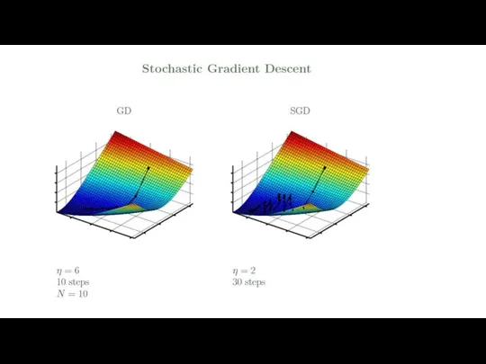
- 4. Gradient descent is a method of numerical optimization that can be used in many algorithms where
- 5. Gradient Descent is the most common optimization algorithm in machine learning and deep learning. It is
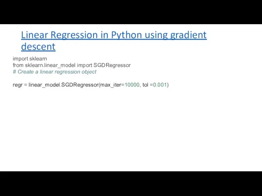
- 8. Linear Regression in Python using gradient descent import sklearn from sklearn.linear_model import SGDRegressor # Create a
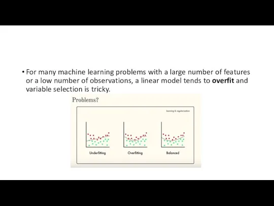
- 9. For many machine learning problems with a large number of features or a low number of
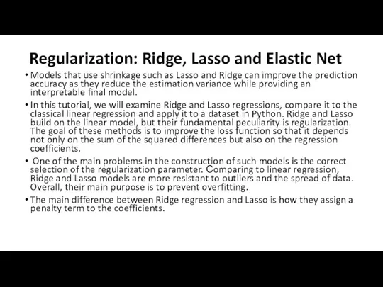
- 10. Regularization: Ridge, Lasso and Elastic Net Models that use shrinkage such as Lasso and Ridge can
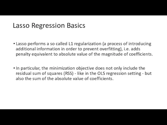
- 11. Lasso Regression Basics Lasso performs a so called L1 regularization (a process of introducing additional information
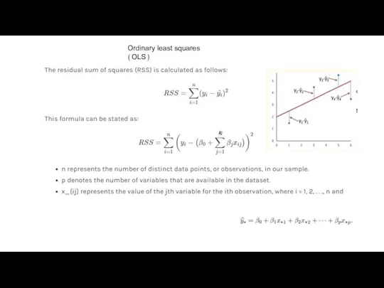
- 12. Ordinary least squares (OLS)
- 14. The LASSO minimizes the sum of squared errors, with an upper bound on the sum of
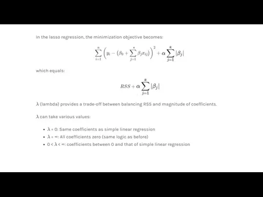
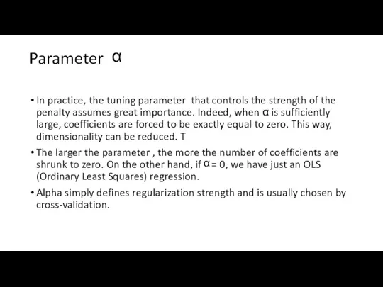
- 15. Parameter In practice, the tuning parameter that controls the strength of the penalty assumes great importance.
- 16. This additional term penalizes the model for having coefficients that do not explain a sufficient amount
- 17. Lasso Regression with Python
- 18. Ridge regression Ridge regression also adds an additional term to the cost function, but instead sums
- 19. rr = Ridge(alpha=0.01) rr.fit(X_train, y_train)
- 20. Elastic Net Elastic Net includes both L-1 and L-2 norm regularization terms. This gives us the
- 21. the elastic net adds a quadratic part to the L1 penalty, which when used alone is
- 22. #Elastic Net model_enet = ElasticNet(alpha = 0.01) model_enet.fit(X_train, y_train)
- 24. Скачать презентацию
Lecture 4.2
Linear Regression.
Linear Regression with Gradient Descent. Regularization
Lecture 4.2
Linear Regression.
Linear Regression with Gradient Descent. Regularization
https://www.youtube.com/watch?v=vMh0zPT0tLI
https://www.youtube.com/watch?v=Q81RR3yKn30
https://www.youtube.com/watch?v=NGf0voTMlcs
https://www.youtube.com/watch?v=1dKRdX9bfIo
https://www.youtube.com/watch?v=Q81RR3yKn30
https://www.youtube.com/watch?v=NGf0voTMlcs
https://www.youtube.com/watch?v=1dKRdX9bfIo
Gradient descent
is a method of numerical optimization that can be used
Gradient descent
is a method of numerical optimization that can be used
Gradient Descent is the most common optimization algorithm in machine learning and deep learning. It
Gradient Descent is the most common optimization algorithm in machine learning and deep learning. It
Linear Regression in Python using gradient descent
import sklearn
from sklearn.linear_model import SGDRegressor
#
Linear Regression in Python using gradient descent
import sklearn
from sklearn.linear_model import SGDRegressor
#
For many machine learning problems with a large number of features
For many machine learning problems with a large number of features
Regularization: Ridge, Lasso and Elastic Net
Models that use shrinkage such as Lasso and
Regularization: Ridge, Lasso and Elastic Net
Models that use shrinkage such as Lasso and
Lasso Regression Basics
Lasso performs a so called L1 regularization (a process
Lasso Regression Basics
Lasso performs a so called L1 regularization (a process
Ordinary least squares (OLS)
Ordinary least squares (OLS)
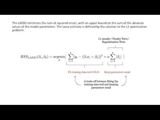
The LASSO minimizes the sum of squared errors, with an upper
The LASSO minimizes the sum of squared errors, with an upper
Parameter
In practice, the tuning parameter that controls the strength of
Parameter
In practice, the tuning parameter that controls the strength of
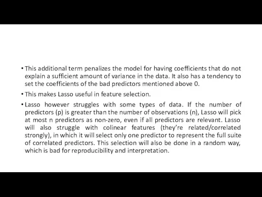
This additional term penalizes the model for having coefficients that do
This additional term penalizes the model for having coefficients that do
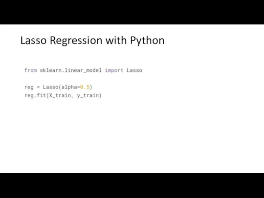
Lasso Regression with Python
Lasso Regression with Python
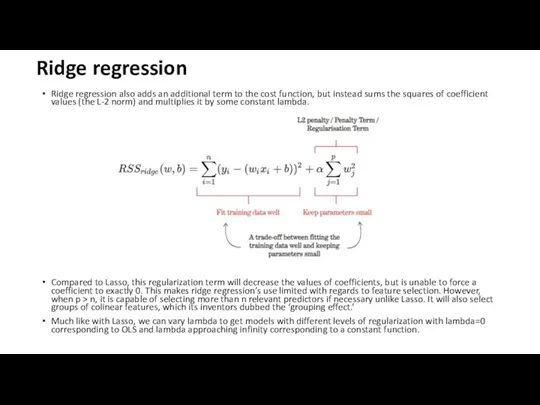
Ridge regression
Ridge regression also adds an additional term to the cost
Ridge regression
Ridge regression also adds an additional term to the cost
rr = Ridge(alpha=0.01)
rr.fit(X_train, y_train)
rr = Ridge(alpha=0.01)
rr.fit(X_train, y_train)
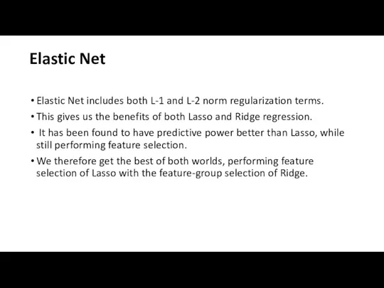
Elastic Net
Elastic Net includes both L-1 and L-2 norm regularization terms.
Elastic Net
Elastic Net includes both L-1 and L-2 norm regularization terms.
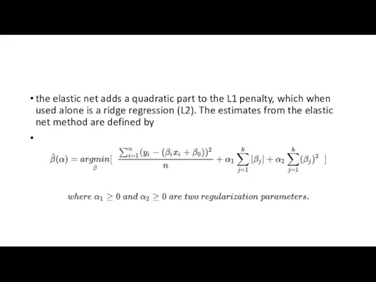
the elastic net adds a quadratic part to the L1 penalty,
the elastic net adds a quadratic part to the L1 penalty,
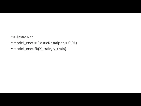
#Elastic Net
model_enet = ElasticNet(alpha = 0.01)
model_enet.fit(X_train, y_train)
#Elastic Net
model_enet = ElasticNet(alpha = 0.01)
model_enet.fit(X_train, y_train)
 Числовые выражения, содержащие знаки + и -
 Математика Путешествие к Робинзону Крузо
 Теорема Пифагора. Пифагор и его школа
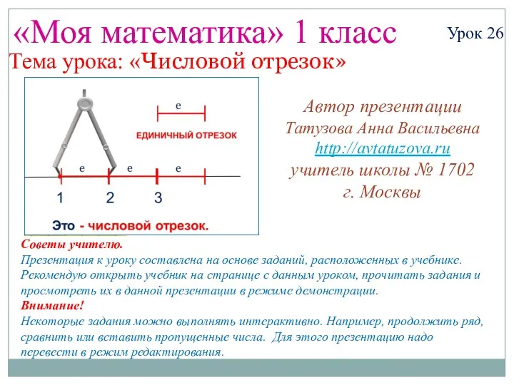 Математика. 1 класс. Урок 26. Числовой отрезок - Презентация
 Число Пи
 Приёмы устных вычислений вида 260+310, 670-140
 Математическая логика и теория алгоритмов
 Отношение порядка. Отношение эквивалентности. (Лекция 8)
 Пирамида
 Формирование вычислительных навыков у учащихся начальной школы
 Пропорция (словарь русского языка Ожегова С.И.)
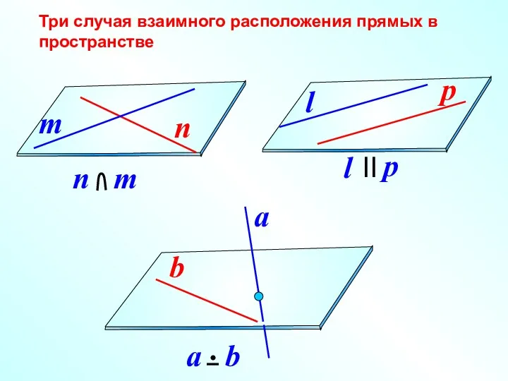 Параллельность прямой и плоскости
 Презентация к уроку математики (2 класс) Тема урока - Деление.
 Решение неравенств с одной переменной
 Сложение и вычитание дробей с одинаковыми знаменателями. Урок математики в 5 классе
 Единицы времени (2 класс)
 конспект урока. ломаная
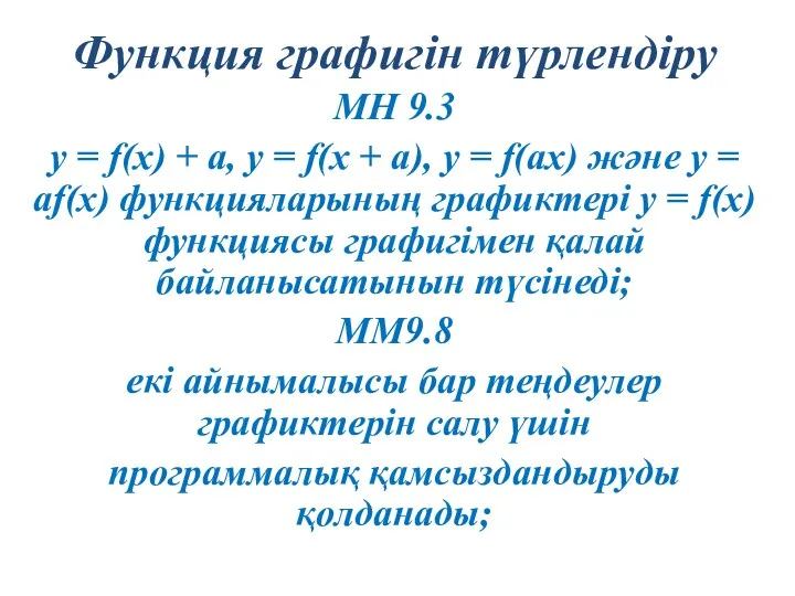 Функция графигін түрлендіру
 Маса. Кілограм (урок № 64)
 История создания величин измерения времени
 Презентация История цифр для 1 класса
 Лекция 2 ЦОС. Преобразование речевых сигналов к цифровому виду
 Все действия с десятичными дробями
 Линейные уравнения с параметрами (7 класс)
 Алгебраические дроби, сокращение дробей
 Последний урок математики в 9 классе
 Свойство квадратного корня
 График линейного уравнения с двумя переменными