- Measures of dispersion. Lecture 3

Содержание
- 2. LECTURE 3 MEASURES OF DISPERSION Saidgozi Saydumarov Sherzodbek Safarov Room: ATB 308 QM Module Leaders Office
- 3. Lecture outline: Range Interquartile range Variance Standard Deviation
- 4. Measures of dispersion Dispersion measures how “spread out” the data is Shows how reliable our conclusions
- 5. Untabulated data
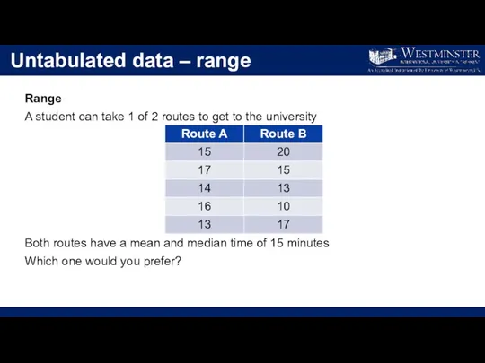
- 6. Untabulated data – range Range A student can take 1 of 2 routes to get to
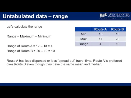
- 7. Untabulated data – range Let’s calculate the range Range = Maximum – Minimum Range of Route
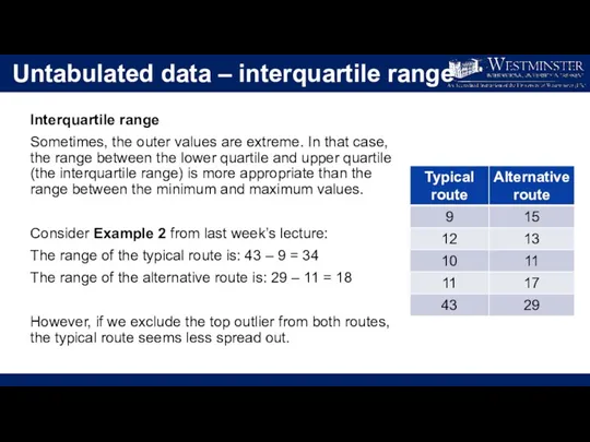
- 8. Untabulated data – interquartile range Interquartile range Sometimes, the outer values are extreme. In that case,
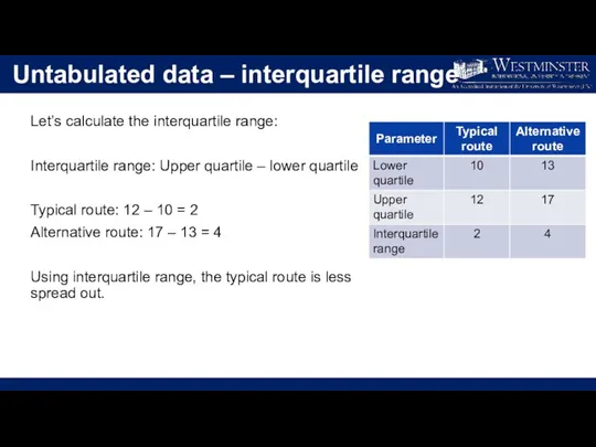
- 9. Untabulated data – interquartile range Let’s calculate the interquartile range: Interquartile range: Upper quartile – lower
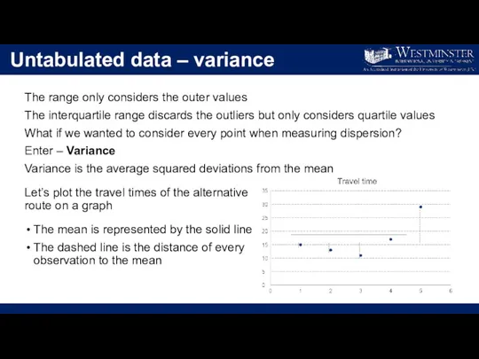
- 10. Untabulated data – variance The range only considers the outer values The interquartile range discards the
- 11. Untabulated data – variance
- 12. Untabulated data – standard deviation
- 13. Tabulated ungrouped data
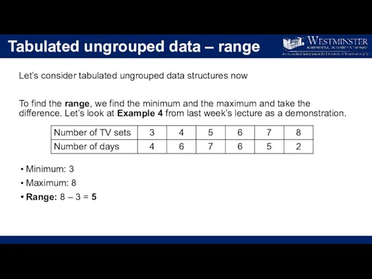
- 14. Tabulated ungrouped data – range Let’s consider tabulated ungrouped data structures now To find the range,
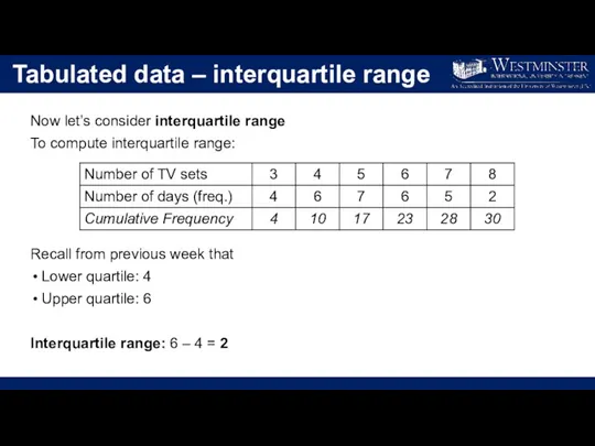
- 15. Tabulated data – interquartile range Now let’s consider interquartile range To compute interquartile range: Recall from
- 16. Tabulated data – variance
- 17. Tabulated grouped data
- 18. Tabulated grouped data - range Let’s consider tabulated grouped data structures The range is still the
- 19. Tabulated data – variance
- 21. Скачать презентацию
LECTURE 3
MEASURES OF DISPERSION
Saidgozi Saydumarov
Sherzodbek Safarov
Room: ATB 308 QM Module Leaders
Office Hours:
LECTURE 3
MEASURES OF DISPERSION
Saidgozi Saydumarov
Sherzodbek Safarov
Room: ATB 308 QM Module Leaders
Office Hours:
Lecture outline:
Range
Interquartile range
Variance
Standard Deviation
Lecture outline:
Range
Interquartile range
Variance
Standard Deviation
Measures of dispersion
Dispersion measures how “spread out” the data is
Shows how
Measures of dispersion
Dispersion measures how “spread out” the data is
Shows how
Untabulated data
Untabulated data
Untabulated data – range
Range
A student can take 1 of 2
Untabulated data – range
Range
A student can take 1 of 2
Untabulated data – range
Let’s calculate the range
Range = Maximum –
Untabulated data – range
Let’s calculate the range
Range = Maximum –
Untabulated data – interquartile range
Interquartile range
Sometimes, the outer values are extreme.
Untabulated data – interquartile range
Interquartile range
Sometimes, the outer values are extreme.
Untabulated data – interquartile range
Let’s calculate the interquartile range:
Interquartile range: Upper
Untabulated data – interquartile range
Let’s calculate the interquartile range:
Interquartile range: Upper
Untabulated data – variance
The range only considers the outer values
The
Untabulated data – variance
The range only considers the outer values
The
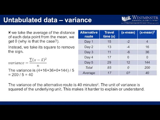
Untabulated data – variance
Untabulated data – variance
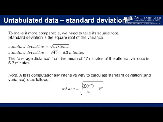
Untabulated data – standard deviation
Untabulated data – standard deviation
Tabulated ungrouped data
Tabulated ungrouped data
Tabulated ungrouped data – range
Let’s consider tabulated ungrouped data structures
Tabulated ungrouped data – range
Let’s consider tabulated ungrouped data structures
Tabulated data – interquartile range
Now let’s consider interquartile range
To compute
Tabulated data – interquartile range
Now let’s consider interquartile range
To compute
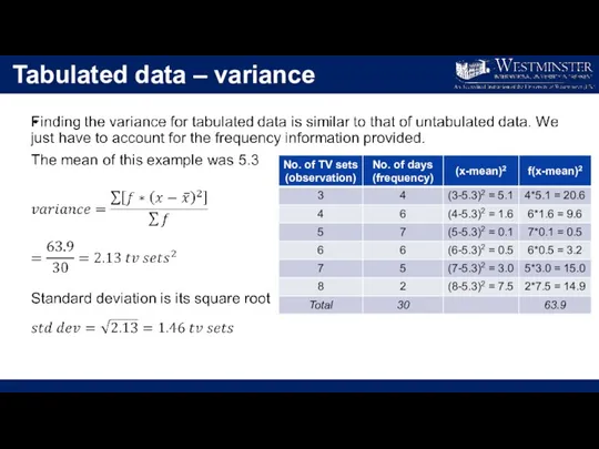
Tabulated data – variance
Tabulated data – variance
Tabulated grouped data
Tabulated grouped data
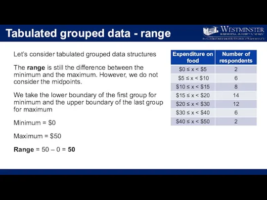
Tabulated grouped data - range
Let’s consider tabulated grouped data structures
The range
Tabulated grouped data - range
Let’s consider tabulated grouped data structures
The range
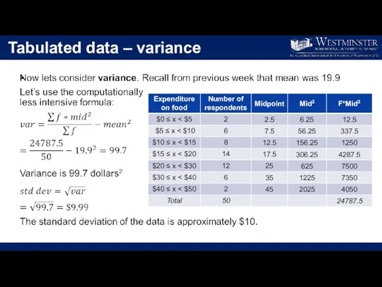
Tabulated data – variance
Tabulated data – variance
 Проверка статистических гипотез
 Графоаналитические методы оценки параметров распределения (лекция 5)
 домашняя
 Теорема Пифагора
 Чтение многозначных чисел
 Pravilnye_Mnogogranniki
 Решение задач в 2 действия
 Пропорция. Отношение
 Сказка – игра Волшебное число по теме: Решение уравнений 5 класс
 Итоговый контрольный тест по геометрии, 7 класс
 Теоретические основы математической логики
 ЕГЭ по математике - 2012. Решаем B13
 Lekciya_14_Ischislenie_predikatov (1)
 Задачи по математике 5 класс
 Конспект открытого мультимедийного урока математики в 4 классе по учебнику Л.Г.Петерсон
 Нахождение числа по заданному значению его дроби
 Наибольший общий делитель. Взаимно простые числа
 Пирамида. Правильная пирамида
 Векторы в пространстве
 Касательная. Уравнение касательной. 10 класс
 Математика: признаки делимости
 Теореми додавання і множення ймовірностей та їх наслідки
 Комбинаторные задачи. Комбинаторика
 Число 9, цифра 9
 Многогранники
 Презентация устный счет 2 класс
 Подготовка к контрольной работе. Многогранники
 Теория вероятности