Measuring Inequality. An examination of the purpose and techniques of inequality measurement презентация
- Measuring Inequality. An examination of the purpose and techniques of inequality measurement

Содержание
- 2. in·equal·i·ty Function: noun 1 : the quality of being unequal or uneven: as a : lack
- 3. Our primary interest is in economic inequality. In this context, inequality measures the disparity between a
- 4. If a single person holds all of a given resource, inequality is at a maximum. If
- 5. Physical attributes – distribution of natural ability is not equal Personal Preferences – Relative valuation of
- 6. Why measure Inequality? Measuring changes in inequality helps determine the effectiveness of policies aimed at affecting
- 7. How do we measure Inequality? Before choosing an inequality measure, the researcher must ask two additional
- 8. Choosing the best metric Range Range Ratio The McLoone Index The Coefficient of Variation The Gini
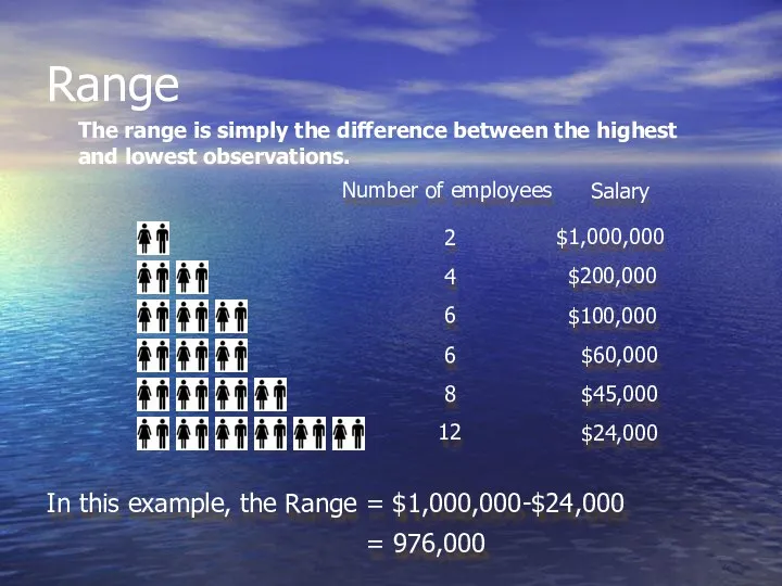
- 9. Range The range is simply the difference between the highest and lowest observations. Number of employees
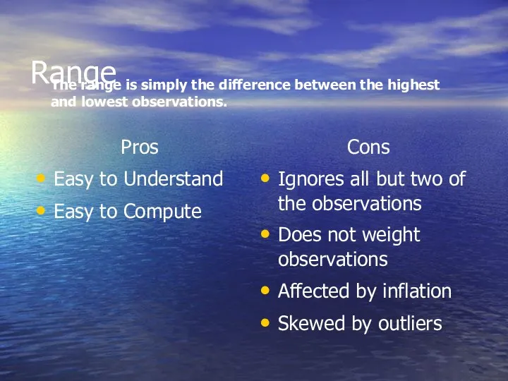
- 10. Range Pros Easy to Understand Easy to Compute Cons Ignores all but two of the observations
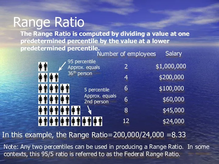
- 11. Range Ratio The Range Ratio is computed by dividing a value at one predetermined percentile by
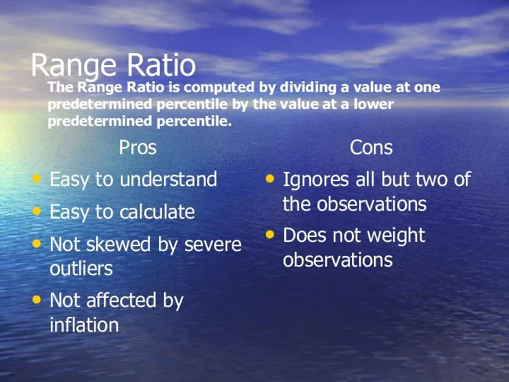
- 12. Range Ratio Pros Easy to understand Easy to calculate Not skewed by severe outliers Not affected
- 13. The McLoone Index The McLoone Index divides the summation of all observations below the median, by
- 14. The McLoone Index Pros Easy to understand Conveys comprehensive information about the bottom half Cons Ignores
- 15. The Coefficient of Variation The Coefficient of Variation is a distribution’s standard deviation divided by its
- 16. The Coefficient of Variation Pros Fairly easy to understand If data is weighted, it is immune
- 17. The Gini Coefficient The Gini Coefficient has an intuitive, but possibly unfamiliar construction. To understand the
- 18. A – Equality Diagonal Population = Income B – Lorenz Curve C – Difference Between Equality
- 19. The Gini Coefficient Mathematically, the Gini Coefficient is equal to twice the area enclosed between the
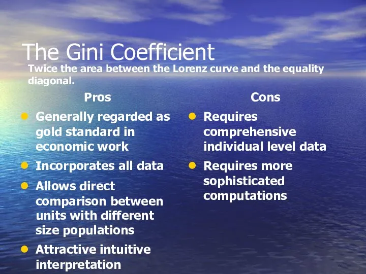
- 20. The Gini Coefficient Pros Generally regarded as gold standard in economic work Incorporates all data Allows
- 21. Theil’s T Statistic Theil’s T Statistic lacks an intuitive picture and involves more than a simple
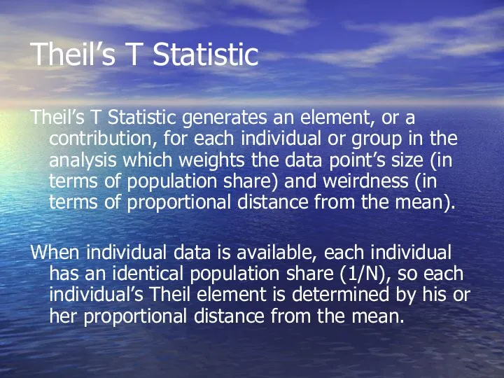
- 22. Theil’s T Statistic Theil’s T Statistic generates an element, or a contribution, for each individual or
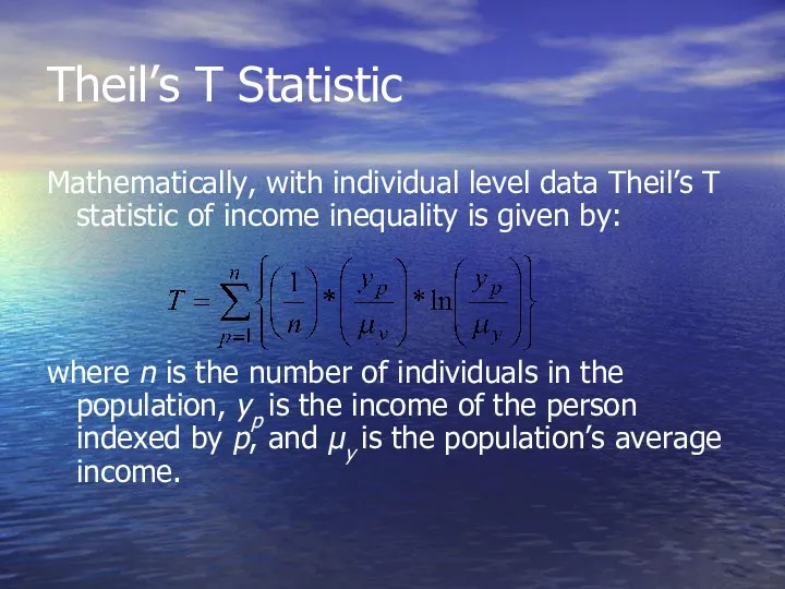
- 23. Theil’s T Statistic Mathematically, with individual level data Theil’s T statistic of income inequality is given
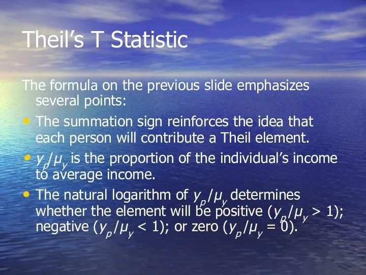
- 24. Theil’s T Statistic The formula on the previous slide emphasizes several points: The summation sign reinforces
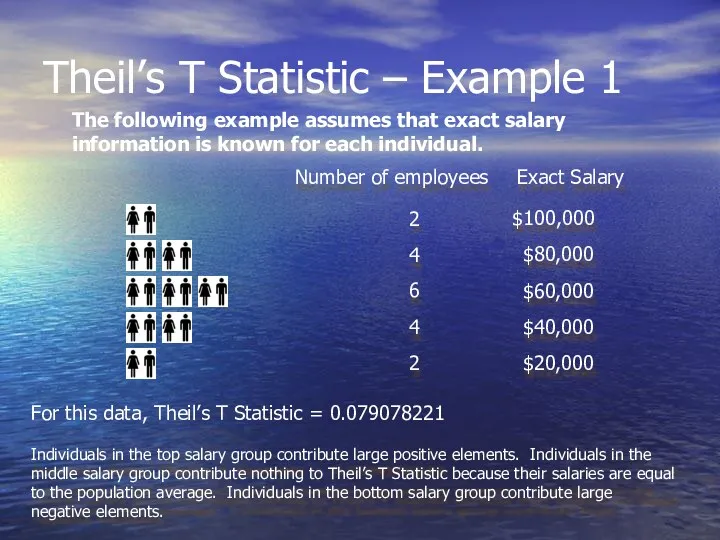
- 25. Theil’s T Statistic – Example 1 The following example assumes that exact salary information is known
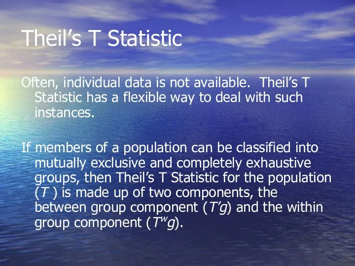
- 26. Theil’s T Statistic Often, individual data is not available. Theil’s T Statistic has a flexible way
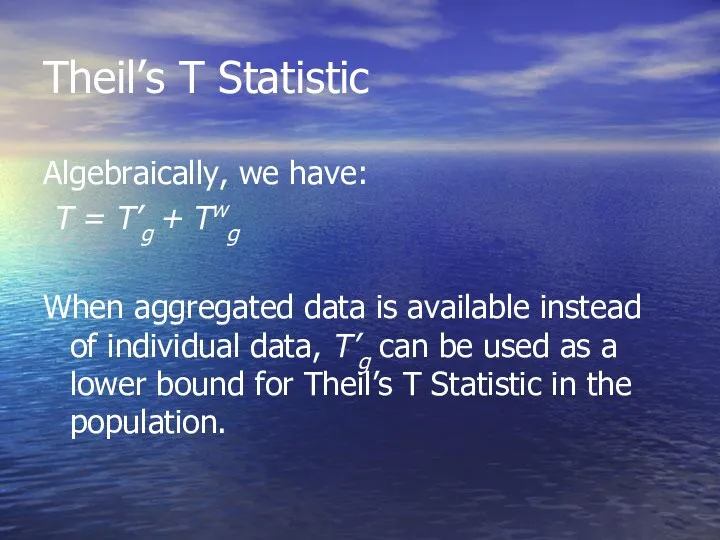
- 27. Theil’s T Statistic Algebraically, we have: T = T’g + Twg When aggregated data is available
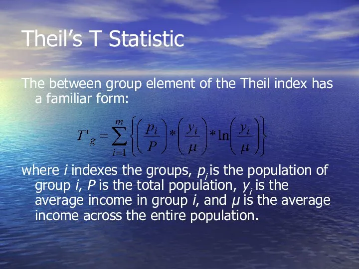
- 28. Theil’s T Statistic The between group element of the Theil index has a familiar form: where
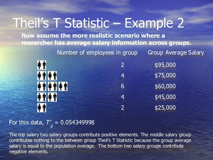
- 29. Theil’s T Statistic – Example 2 Now assume the more realistic scenario where a researcher has
- 30. Group analysis with Theil’s T Statistic: As Example 2 hints, Theil’s T Statistic is a powerful
- 31. Theil’s T Statistic Pros Can effectively use group data Allows the researcher to parse inequality into
- 33. Скачать презентацию
in·equal·i·ty
Function: noun
1 : the quality of being unequal or uneven:
in·equal·i·ty Function: noun 1 : the quality of being unequal or uneven:

Our primary interest is in economic inequality.
In this context, inequality measures
Our primary interest is in economic inequality.
In this context, inequality measures

If a single person holds all of a given resource, inequality
If a single person holds all of a given resource, inequality
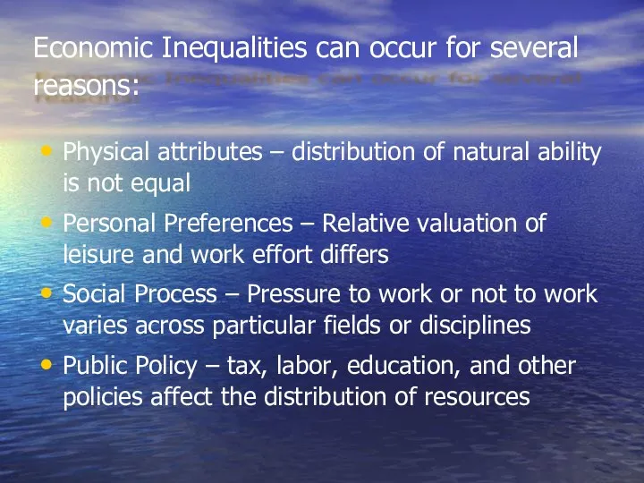
Physical attributes – distribution of natural ability is not equal
Personal Preferences
Physical attributes – distribution of natural ability is not equal
Personal Preferences

Why measure Inequality?
Measuring changes in inequality helps determine the effectiveness of
Why measure Inequality?
Measuring changes in inequality helps determine the effectiveness of
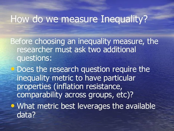
How do we measure Inequality?
Before choosing an inequality measure, the researcher
How do we measure Inequality?
Before choosing an inequality measure, the researcher
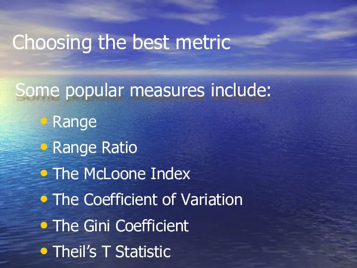
Choosing the best metric
Range
Range Ratio
The McLoone Index
The Coefficient of Variation
The
Choosing the best metric
Range
Range Ratio
The McLoone Index
The Coefficient of Variation
The
Range
The range is simply the difference between the highest and lowest
Range
The range is simply the difference between the highest and lowest
Range
Pros
Easy to Understand
Easy to Compute
Cons
Ignores all but two of the observations
Does
Range
Pros
Easy to Understand
Easy to Compute
Cons
Ignores all but two of the observations
Does
Range Ratio
The Range Ratio is computed by dividing a value at
Range Ratio
The Range Ratio is computed by dividing a value at
Range Ratio
Pros
Easy to understand
Easy to calculate
Not skewed by severe outliers
Not affected
Range Ratio
Pros
Easy to understand
Easy to calculate
Not skewed by severe outliers
Not affected
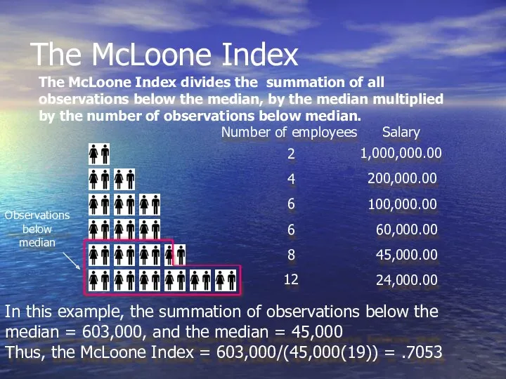
The McLoone Index
The McLoone Index divides the summation of all observations
The McLoone Index
The McLoone Index divides the summation of all observations
The McLoone Index
Pros
Easy to understand
Conveys comprehensive information about the bottom half
Cons
Ignores
The McLoone Index
Pros
Easy to understand
Conveys comprehensive information about the bottom half
Cons
Ignores
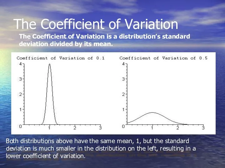
The Coefficient of Variation
The Coefficient of Variation is a distribution’s standard
The Coefficient of Variation
The Coefficient of Variation is a distribution’s standard
The Coefficient of Variation
Pros
Fairly easy to understand
If data is weighted, it
The Coefficient of Variation
Pros
Fairly easy to understand
If data is weighted, it

The Gini Coefficient
The Gini Coefficient has an intuitive, but possibly unfamiliar
The Gini Coefficient
The Gini Coefficient has an intuitive, but possibly unfamiliar
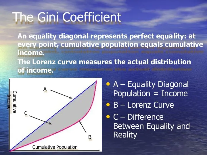
A – Equality Diagonal Population = Income
B – Lorenz Curve
C
A – Equality Diagonal Population = Income
B – Lorenz Curve
C
The Gini Coefficient
Mathematically, the Gini Coefficient is equal to twice the
The Gini Coefficient
Mathematically, the Gini Coefficient is equal to twice the
The Gini Coefficient
Pros
Generally regarded as gold standard in economic work
Incorporates all
The Gini Coefficient
Pros
Generally regarded as gold standard in economic work
Incorporates all
Theil’s T Statistic
Theil’s T Statistic lacks an intuitive picture and involves
Theil’s T Statistic
Theil’s T Statistic lacks an intuitive picture and involves
Theil’s T Statistic
Theil’s T Statistic generates an element, or a contribution,
Theil’s T Statistic
Theil’s T Statistic generates an element, or a contribution,
Theil’s T Statistic
Mathematically, with individual level data Theil’s T statistic of
Theil’s T Statistic
Mathematically, with individual level data Theil’s T statistic of
Theil’s T Statistic
The formula on the previous slide emphasizes several points:
The
Theil’s T Statistic
The formula on the previous slide emphasizes several points:
The
Theil’s T Statistic – Example 1
The following example assumes that exact
Theil’s T Statistic – Example 1
The following example assumes that exact
Theil’s T Statistic
Often, individual data is not available. Theil’s T Statistic
Theil’s T Statistic
Often, individual data is not available. Theil’s T Statistic
Theil’s T Statistic
Algebraically, we have:
T = T’g + Twg
When
Theil’s T Statistic
Algebraically, we have:
T = T’g + Twg
When
Theil’s T Statistic
The between group element of the Theil index has
Theil’s T Statistic
The between group element of the Theil index has
Theil’s T Statistic – Example 2
Now assume the more realistic scenario
Theil’s T Statistic – Example 2
Now assume the more realistic scenario
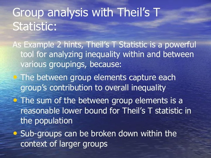
Group analysis with Theil’s T Statistic:
As Example 2 hints, Theil’s T
Group analysis with Theil’s T Statistic:
As Example 2 hints, Theil’s T
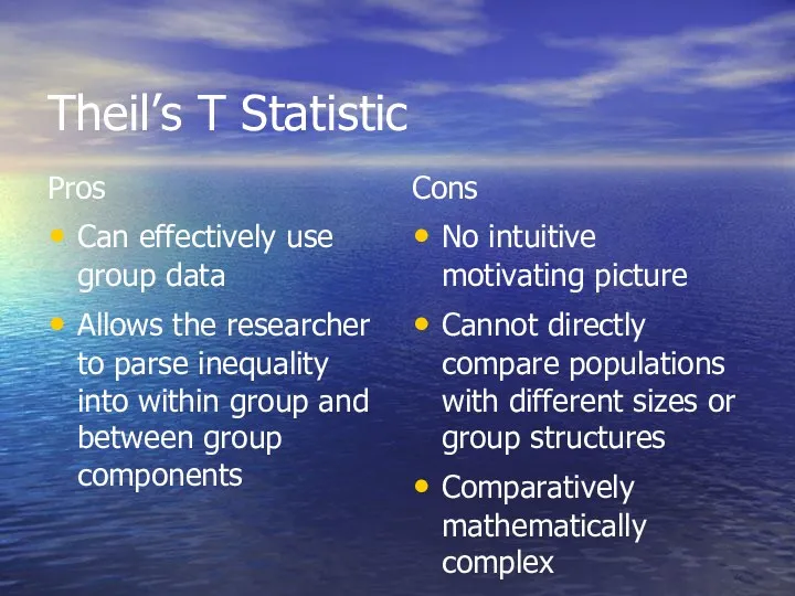
Theil’s T Statistic
Pros
Can effectively use group data
Allows the researcher to parse
Theil’s T Statistic
Pros
Can effectively use group data
Allows the researcher to parse
 Review of Basic Concepts in Statistics
 Треугольник. Признаки равенства треугольников
 Перпендикуляр и наклонные. Расстояние от точки до плоскости
 Від’ємні числа, дії над ними
 Сравнение дробей
 Тест по теме: Призма. Часть 2. Вариант 1
 Методы и системы поддержки принятия решений. Многокритериальный анализ решений: лексикографический метод, обобщенные критерии
 Графы. Основные понятия
 Анализируем результаты ЕГЭ 15, готовимся к ЕГЭ 16
 Тригонометрические неравенства
 Признаки параллельности прямых. 7 класс
 презентация к уроку по математике Единицы времени. Год
 Графики тригонометрических функций
 Признаки делимости натуральных чисел. Практикум по решению задания №19 ЕГЭ (базовый уровень)
 Презентация к открытому уроку по математике для 1 класса по теме:Секрет сложения.
 Округление натуральных чисел
 Быстрее. Выше. Сильнее. Тренажёр по математике
 Презентация для урока математики в 1 классе. Устный счет
 Урок математики(1класс)
 Деление (математика, 3 класс, УМК Гармония)
 Решение задач на составление уравнений
 Пропорциональные отрезки в прямоугольном треугольнике
 Игра-тренажёр В гостях у ёжика (математика 1 класс)
 Корреляционно-регрессионный анализ
 Теорема П'єра Ферма
 Основы математического анализа
 Решение планиметрических многовариантных задач
 Птицы из красной книги Башкортостана. Региональный компонент на уроках математики в начальной школе