- Probabilistic Models. Chapter 11

Содержание
- 2. Types of Probability Fundamentals of Probability Statistical Independence and Dependence Expected Value The Normal Distribution Chapter
- 3. Deterministic techniques assume that no uncertainty exists in model parameters. Chapters 2-10 introduced topics that are
- 4. Classical, or a priori (prior to the occurrence), probability is an objective probability that can be
- 5. Subjective probability is an estimate based on personal belief, experience, or knowledge of a situation. It
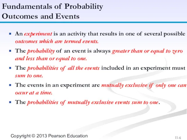
- 6. An experiment is an activity that results in one of several possible outcomes which are termed
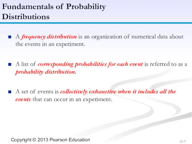
- 7. A frequency distribution is an organization of numerical data about the events in an experiment. A
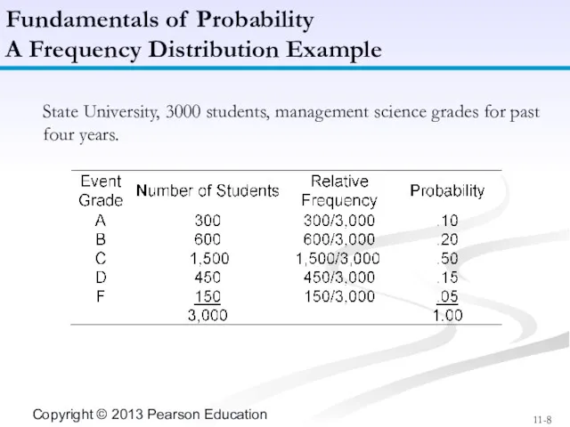
- 8. State University, 3000 students, management science grades for past four years. Fundamentals of Probability A Frequency
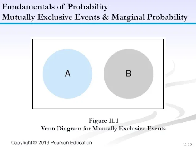
- 9. A marginal probability is the probability of a single event occurring, denoted by P(A). For mutually
- 10. Figure 11.1 Venn Diagram for Mutually Exclusive Events Fundamentals of Probability Mutually Exclusive Events & Marginal
- 11. Probability that non-mutually exclusive events A and B or both will occur expressed as: P(A or
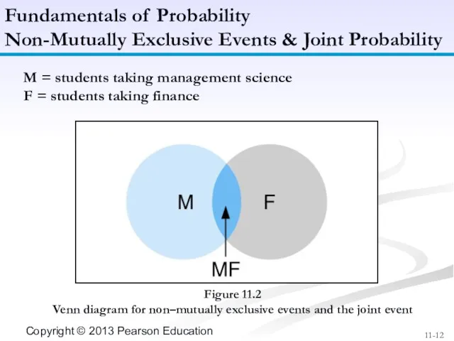
- 12. Figure 11.2 Venn diagram for non–mutually exclusive events and the joint event Fundamentals of Probability Non-Mutually
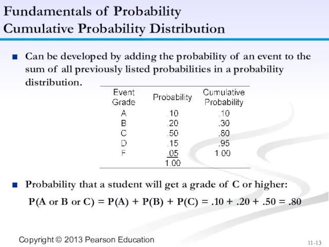
- 13. Can be developed by adding the probability of an event to the sum of all previously
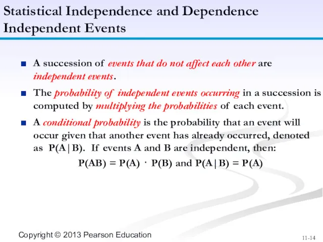
- 14. A succession of events that do not affect each other are independent events. The probability of
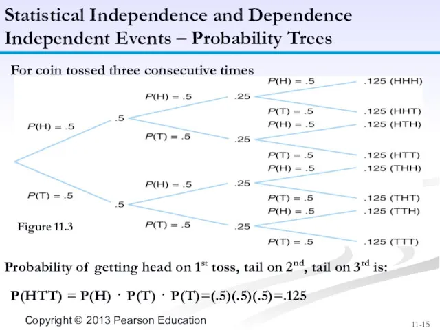
- 15. For coin tossed three consecutive times Figure 11.3 Statistical Independence and Dependence Independent Events – Probability
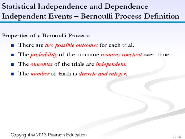
- 16. Properties of a Bernoulli Process: There are two possible outcomes for each trial. The probability of
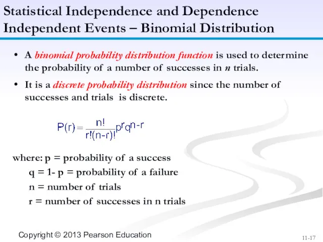
- 17. A binomial probability distribution function is used to determine the probability of a number of successes
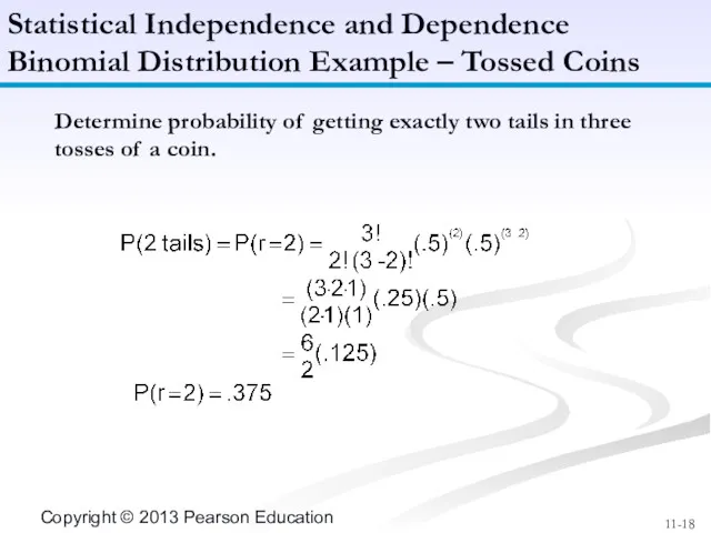
- 18. Determine probability of getting exactly two tails in three tosses of a coin. Statistical Independence and
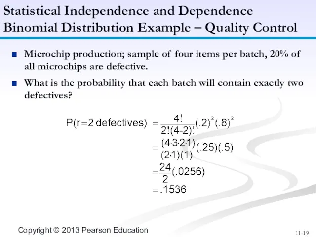
- 19. Microchip production; sample of four items per batch, 20% of all microchips are defective. What is
- 20. Four microchips tested per batch; if two or more found defective, batch is rejected. What is
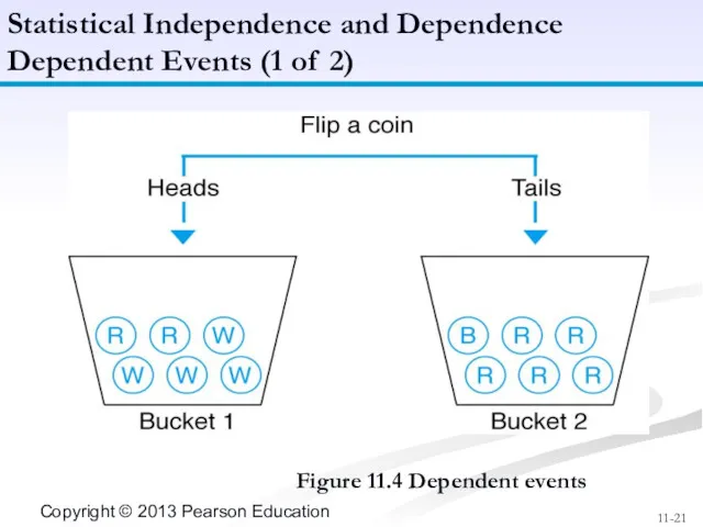
- 21. Figure 11.4 Dependent events Statistical Independence and Dependence Dependent Events (1 of 2)
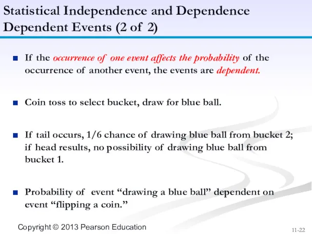
- 22. If the occurrence of one event affects the probability of the occurrence of another event, the
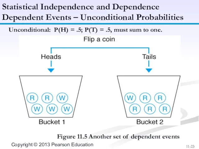
- 23. Unconditional: P(H) = .5; P(T) = .5, must sum to one. Figure 11.5 Another set of
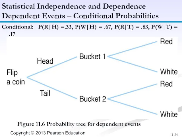
- 24. Conditional: P(R|H) =.33, P(W|H) = .67, P(R|T) = .83, P(W|T) = .17 Statistical Independence and Dependence
- 25. Given two dependent events A and B: P(A|B) = P(AB)/P(B) With data from previous example: P(RH)
- 26. Figure 11.7 Probability tree with marginal, conditional and joint probabilities Statistical Independence and Dependence Summary of
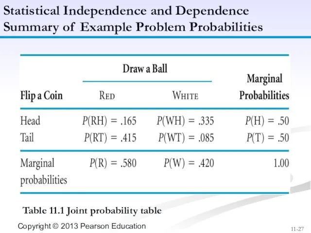
- 27. Table 11.1 Joint probability table Statistical Independence and Dependence Summary of Example Problem Probabilities
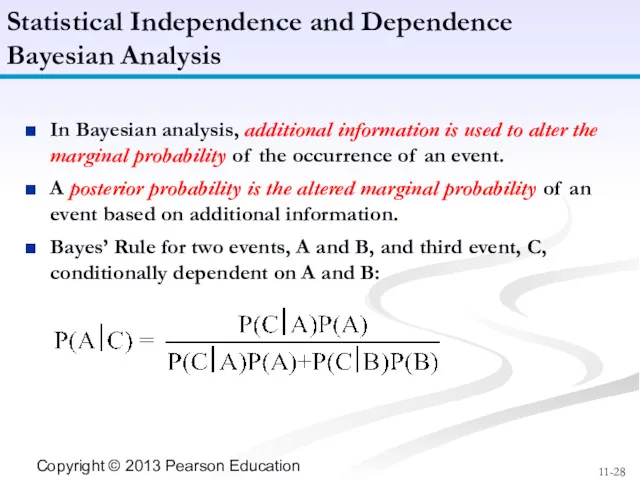
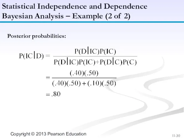
- 28. In Bayesian analysis, additional information is used to alter the marginal probability of the occurrence of
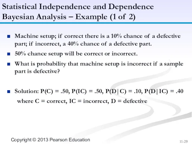
- 29. Machine setup; if correct there is a 10% chance of a defective part; if incorrect, a
- 30. Posterior probabilities: Statistical Independence and Dependence Bayesian Analysis – Example (2 of 2)
- 31. When the values of variables occur in no particular order or sequence, the variables are referred
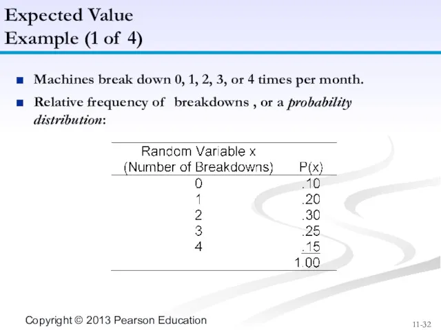
- 32. Machines break down 0, 1, 2, 3, or 4 times per month. Relative frequency of breakdowns
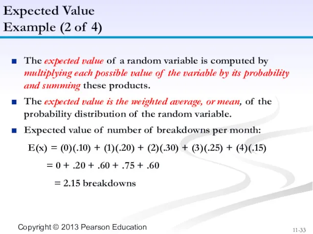
- 33. The expected value of a random variable is computed by multiplying each possible value of the
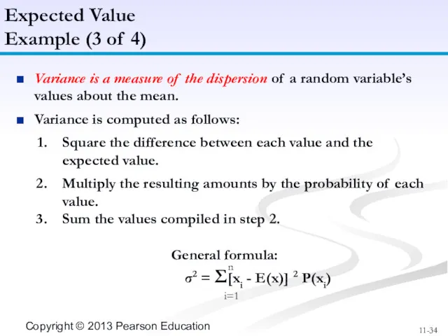
- 34. Variance is a measure of the dispersion of a random variable’s values about the mean. Variance
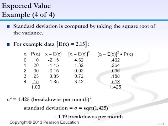
- 35. Standard deviation is computed by taking the square root of the variance. For example data [E(x)
- 36. A continuous random variable can take on an infinite number of values within some interval. Continuous
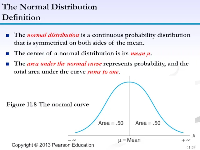
- 37. The normal distribution is a continuous probability distribution that is symmetrical on both sides of the
- 38. Mean weekly carpet sales of 4,200 yards, with a standard deviation of 1,400 yards. What is
- 39. - - Figure 11.9 The normal distribution for carpet demand The Normal Distribution Example (2 of
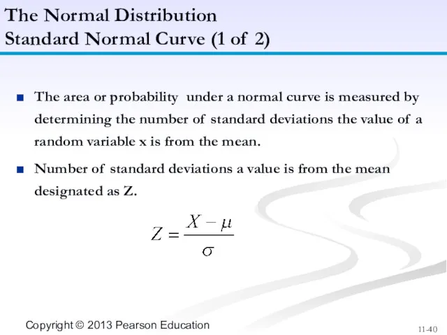
- 40. The area or probability under a normal curve is measured by determining the number of standard
- 41. The Normal Distribution Standard Normal Curve (2 of 2) Figure 11.10 The standard normal distribution
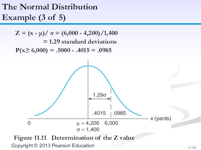
- 42. Figure 11.11 Determination of the Z value The Normal Distribution Example (3 of 5) Z =
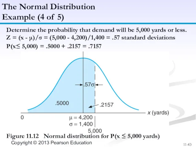
- 43. Determine the probability that demand will be 5,000 yards or less. Z = (x - μ)/σ
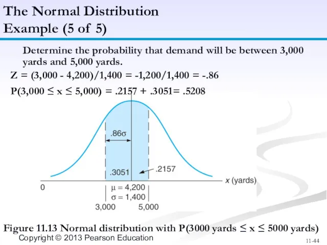
- 44. The Normal Distribution Example (5 of 5) Figure 11.13 Normal distribution with P(3000 yards ≤ x
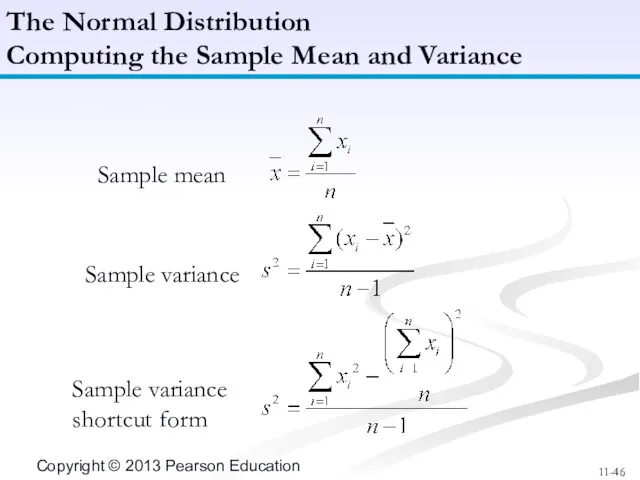
- 45. The population mean and variance are for the entire set of data being analyzed. The sample
- 46. The Normal Distribution Computing the Sample Mean and Variance Sample mean Sample variance Sample variance shortcut
- 47. Sample mean = 42,000/10 = 4,200 yd Sample variance = [(190,060,000) - (1,764,000,000/10)]/9 = 1,517,777 Sample
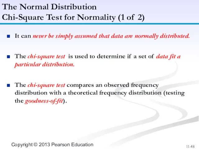
- 48. It can never be simply assumed that data are normally distributed. The chi-square test is used
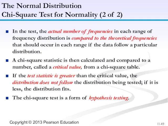
- 49. In the test, the actual number of frequencies in each range of frequency distribution is compared
- 50. Armor Carpet Store example - assume sample mean = 4,200 yards, and sample standard deviation =1,232
- 51. Figure 11.14 The theoretical normal distribution The Normal Distribution Example of Chi-Square Test (2 of 6)
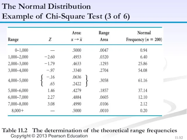
- 52. Table 11.2 The determination of the theoretical range frequencies The Normal Distribution Example of Chi-Square Test
- 53. The Normal Distribution Example of Chi-Square Test (4 of 6) Comparing theoretical frequencies with actual frequencies:
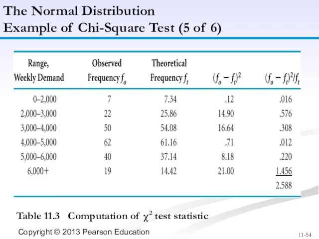
- 54. Table 11.3 Computation of χ2 test statistic The Normal Distribution Example of Chi-Square Test (5 of
- 55. χ2k-p-1 = Σ(fo - ft)2/10 = 2.588 k - p -1 = 6 - 2 –
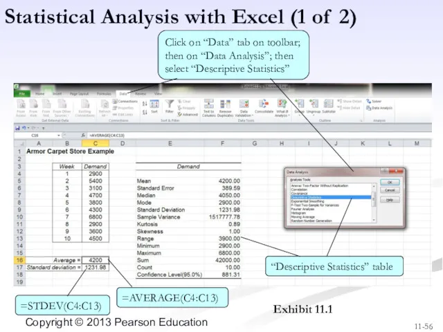
- 56. Exhibit 11.1 Statistical Analysis with Excel (1 of 2) Click on “Data” tab on toolbar; then
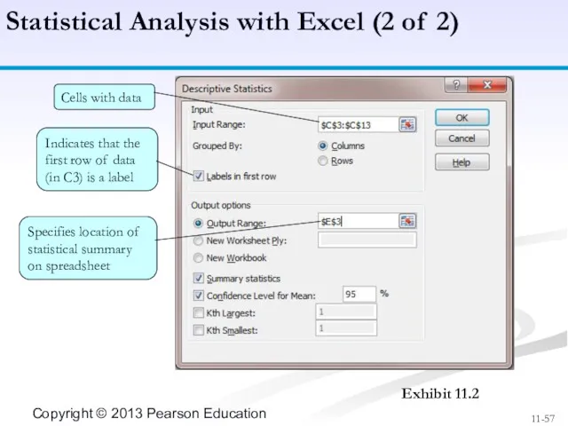
- 57. Statistical Analysis with Excel (2 of 2) Exhibit 11.2 Cells with data Indicates that the first
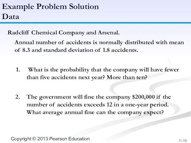
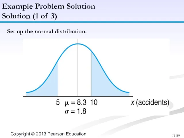
- 58. Radcliff Chemical Company and Arsenal. Annual number of accidents is normally distributed with mean of 8.3
- 59. Set up the normal distribution. Example Problem Solution Solution (1 of 3)
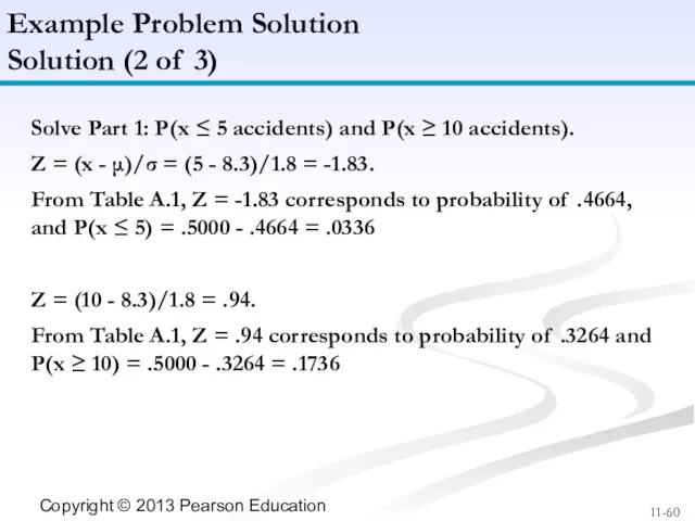
- 60. Solve Part 1: P(x ≤ 5 accidents) and P(x ≥ 10 accidents). Z = (x -
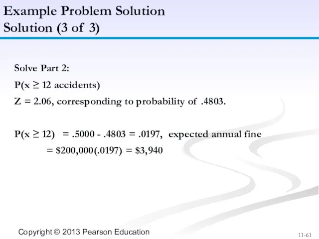
- 61. Solve Part 2: P(x ≥ 12 accidents) Z = 2.06, corresponding to probability of .4803. P(x
- 63. Скачать презентацию
Types of Probability
Fundamentals of Probability
Statistical Independence and Dependence
Expected Value
The Normal Distribution
Chapter Topics
Types of Probability
Fundamentals of Probability
Statistical Independence and Dependence
Expected Value
The Normal Distribution
Chapter Topics
Deterministic techniques assume that no uncertainty exists in model parameters. Chapters 2-10 introduced
Deterministic techniques assume that no uncertainty exists in model parameters. Chapters 2-10 introduced
Classical, or a priori (prior to the occurrence), probability is an objective probability
Classical, or a priori (prior to the occurrence), probability is an objective probability
Subjective probability is an estimate based on personal belief, experience, or knowledge of
Subjective probability is an estimate based on personal belief, experience, or knowledge of
An experiment is an activity that results in one of several possible outcomes
An experiment is an activity that results in one of several possible outcomes
A frequency distribution is an organization of numerical data about the events in
A frequency distribution is an organization of numerical data about the events in
State University, 3000 students, management science grades for past four years.
Fundamentals of Probability
A
State University, 3000 students, management science grades for past four years.
Fundamentals of Probability
A
A marginal probability is the probability of a single event occurring, denoted by
A marginal probability is the probability of a single event occurring, denoted by
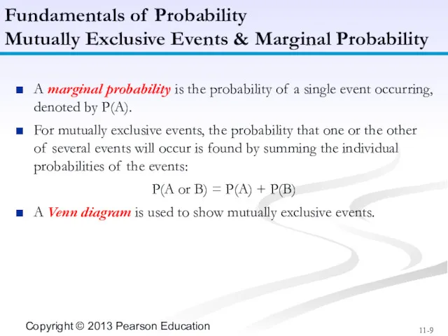
Figure 11.1
Venn Diagram for Mutually Exclusive Events
Fundamentals of Probability
Mutually Exclusive Events & Marginal
Figure 11.1
Venn Diagram for Mutually Exclusive Events
Fundamentals of Probability
Mutually Exclusive Events & Marginal
Probability that non-mutually exclusive events A and B or both will occur expressed
Probability that non-mutually exclusive events A and B or both will occur expressed
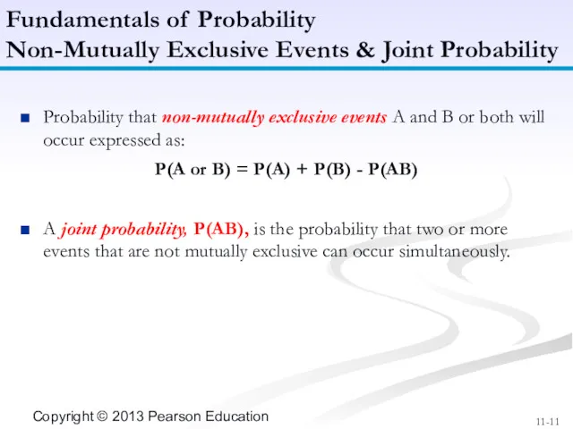
Figure 11.2
Venn diagram for non–mutually exclusive events and the joint event
Fundamentals of Probability
Non-Mutually
Figure 11.2
Venn diagram for non–mutually exclusive events and the joint event
Fundamentals of Probability
Non-Mutually
Can be developed by adding the probability of an event to the sum
Can be developed by adding the probability of an event to the sum
A succession of events that do not affect each other are independent events.
The
A succession of events that do not affect each other are independent events.
The
For coin tossed three consecutive times
Figure 11.3
Statistical Independence and Dependence
Independent Events – Probability
For coin tossed three consecutive times
Figure 11.3
Statistical Independence and Dependence
Independent Events – Probability
Properties of a Bernoulli Process:
There are two possible outcomes for each trial.
Properties of a Bernoulli Process:
There are two possible outcomes for each trial.
A binomial probability distribution function is used to determine the probability of a
A binomial probability distribution function is used to determine the probability of a
Determine probability of getting exactly two tails in three tosses of a coin.
Determine probability of getting exactly two tails in three tosses of a coin.
Microchip production; sample of four items per batch, 20% of all microchips are
Microchip production; sample of four items per batch, 20% of all microchips are
Four microchips tested per batch; if two or more found defective, batch is
Four microchips tested per batch; if two or more found defective, batch is
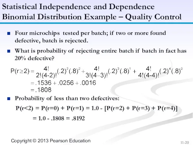
Figure 11.4 Dependent events
Statistical Independence and Dependence
Dependent Events (1 of 2)
Figure 11.4 Dependent events
Statistical Independence and Dependence
Dependent Events (1 of 2)
If the occurrence of one event affects the probability of the occurrence of
If the occurrence of one event affects the probability of the occurrence of
Unconditional: P(H) = .5; P(T) = .5, must sum to one.
Figure 11.5 Another
Unconditional: P(H) = .5; P(T) = .5, must sum to one.
Figure 11.5 Another
Conditional: P(R|H) =.33, P(W|H) = .67, P(R|T) = .83, P(W|T) = .17
Statistical Independence
Conditional: P(R|H) =.33, P(W|H) = .67, P(R|T) = .83, P(W|T) = .17
Statistical Independence
Given two dependent events A and B:
P(A|B) = P(AB)/P(B)
With data from previous example:
P(RH)
Given two dependent events A and B:
P(A|B) = P(AB)/P(B)
With data from previous example:
P(RH)
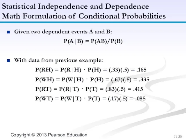
Figure 11.7 Probability tree with marginal, conditional and joint probabilities
Statistical Independence and Dependence
Summary
Figure 11.7 Probability tree with marginal, conditional and joint probabilities
Statistical Independence and Dependence
Summary
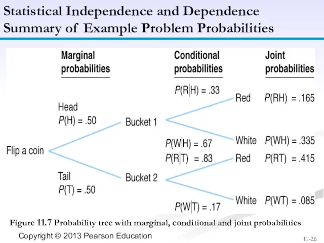
Table 11.1 Joint probability table
Statistical Independence and Dependence
Summary of Example Problem Probabilities
Table 11.1 Joint probability table
Statistical Independence and Dependence
Summary of Example Problem Probabilities
In Bayesian analysis, additional information is used to alter the marginal probability of
In Bayesian analysis, additional information is used to alter the marginal probability of
Machine setup; if correct there is a 10% chance of a defective part;
Machine setup; if correct there is a 10% chance of a defective part;
Posterior probabilities:
Statistical Independence and Dependence
Bayesian Analysis – Example (2 of 2)
Posterior probabilities:
Statistical Independence and Dependence
Bayesian Analysis – Example (2 of 2)
When the values of variables occur in no particular order or sequence, the
When the values of variables occur in no particular order or sequence, the
Machines break down 0, 1, 2, 3, or 4 times per month.
Relative frequency
Machines break down 0, 1, 2, 3, or 4 times per month.
Relative frequency
The expected value of a random variable is computed by multiplying each possible
The expected value of a random variable is computed by multiplying each possible
Variance is a measure of the dispersion of a random variable’s values about
Variance is a measure of the dispersion of a random variable’s values about
Standard deviation is computed by taking the square root of the variance.
For example
Standard deviation is computed by taking the square root of the variance.
For example
A continuous random variable can take on an infinite number of values within
A continuous random variable can take on an infinite number of values within
The normal distribution is a continuous probability distribution that is symmetrical on both
The normal distribution is a continuous probability distribution that is symmetrical on both
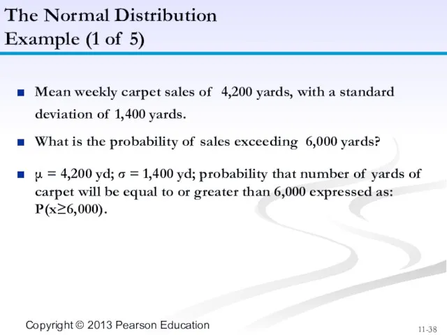
Mean weekly carpet sales of 4,200 yards, with a standard deviation of 1,400
Mean weekly carpet sales of 4,200 yards, with a standard deviation of 1,400
-
-
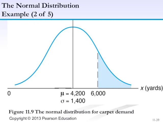
Figure 11.9 The normal distribution for carpet demand
The Normal Distribution
Example (2 of 5)
P(x≥6,000)
-
-
Figure 11.9 The normal distribution for carpet demand
The Normal Distribution
Example (2 of 5)
P(x≥6,000)
The area or probability under a normal curve is measured by determining the
The area or probability under a normal curve is measured by determining the
The Normal Distribution
Standard Normal Curve (2 of 2)
Figure 11.10 The standard normal distribution
The Normal Distribution
Standard Normal Curve (2 of 2)
Figure 11.10 The standard normal distribution
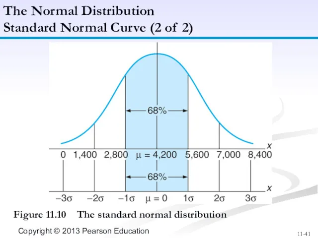
Figure 11.11 Determination of the Z value
The Normal Distribution
Example (3 of 5)
Z =
Figure 11.11 Determination of the Z value
The Normal Distribution
Example (3 of 5)
Z =
Determine the probability that demand will be 5,000 yards or less.
Z = (x
Determine the probability that demand will be 5,000 yards or less.
Z = (x
The Normal Distribution
Example (5 of 5)
Figure 11.13 Normal distribution with P(3000 yards ≤
The Normal Distribution
Example (5 of 5)
Figure 11.13 Normal distribution with P(3000 yards ≤
The population mean and variance are for the entire set of data being
The population mean and variance are for the entire set of data being
The Normal Distribution
Computing the Sample Mean and Variance
Sample mean
Sample variance
Sample variance shortcut form
The Normal Distribution
Computing the Sample Mean and Variance
Sample mean
Sample variance
Sample variance shortcut form
Sample mean = 42,000/10 = 4,200 yd
Sample variance = [(190,060,000) - (1,764,000,000/10)]/9
=
Sample mean = 42,000/10 = 4,200 yd
Sample variance = [(190,060,000) - (1,764,000,000/10)]/9
=
![Sample mean = 42,000/10 = 4,200 yd Sample variance = [(190,060,000) - (1,764,000,000/10)]/9](/_ipx/f_webp&q_80&fit_contain&s_1440x1080/imagesDir/jpg/137870/slide-46.jpg)
It can never be simply assumed that data are normally distributed.
The chi-square test
It can never be simply assumed that data are normally distributed.
The chi-square test
In the test, the actual number of frequencies in each range of frequency
In the test, the actual number of frequencies in each range of frequency
Armor Carpet Store example - assume sample mean = 4,200 yards, and sample
Armor Carpet Store example - assume sample mean = 4,200 yards, and sample
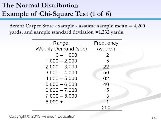
Figure 11.14 The theoretical normal distribution
The Normal Distribution
Example of Chi-Square Test (2 of
Figure 11.14 The theoretical normal distribution
The Normal Distribution
Example of Chi-Square Test (2 of
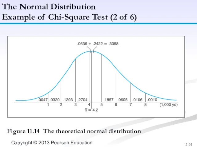
Table 11.2 The determination of the theoretical range frequencies
The Normal Distribution
Example of Chi-Square
Table 11.2 The determination of the theoretical range frequencies
The Normal Distribution
Example of Chi-Square
The Normal Distribution
Example of Chi-Square Test (4 of 6)
Comparing theoretical frequencies with actual
The Normal Distribution
Example of Chi-Square Test (4 of 6)
Comparing theoretical frequencies with actual
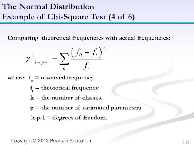
Table 11.3 Computation of χ2 test statistic
The Normal Distribution
Example of Chi-Square Test
Table 11.3 Computation of χ2 test statistic
The Normal Distribution
Example of Chi-Square Test
χ2k-p-1 = Σ(fo - ft)2/10 = 2.588
k - p -1 = 6 -
χ2k-p-1 = Σ(fo - ft)2/10 = 2.588
k - p -1 = 6 -
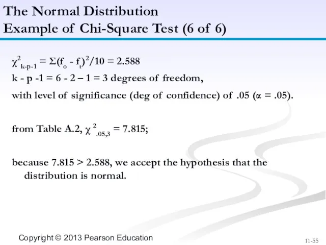
Exhibit 11.1
Statistical Analysis with Excel (1 of 2)
Click on “Data” tab on toolbar;
Exhibit 11.1
Statistical Analysis with Excel (1 of 2)
Click on “Data” tab on toolbar;
Statistical Analysis with Excel (2 of 2)
Exhibit 11.2
Cells with data
Indicates that the first
Statistical Analysis with Excel (2 of 2)
Exhibit 11.2
Cells with data
Indicates that the first
Radcliff Chemical Company and Arsenal.
Annual number of accidents is normally distributed with mean
Radcliff Chemical Company and Arsenal.
Annual number of accidents is normally distributed with mean
Set up the normal distribution.
Example Problem Solution
Solution (1 of 3)
Set up the normal distribution.
Example Problem Solution
Solution (1 of 3)
Solve Part 1: P(x ≤ 5 accidents) and P(x ≥ 10 accidents).
Z =
Solve Part 1: P(x ≤ 5 accidents) and P(x ≥ 10 accidents).
Z =
Solve Part 2:
P(x ≥ 12 accidents)
Z = 2.06, corresponding to probability
Solve Part 2:
P(x ≥ 12 accidents)
Z = 2.06, corresponding to probability
 Описательная статистика в Excel. (Лекция 4)
 Презентация к занятию Казлар - аккошлар әкияте эзләре буйлап
 Математика в жизни человека
 Число 10. Состав числа 10
 Устный счёт.
 Аксиомы стереометрии и их простейшие следствия
 Задачи, раскрывающие смысл действия деления
 Ряд натуральных чисел. Цифры. Десятичная запись натуральных чисел
 Решение полного квадратного уравнения
 Сорбонки. Математика 1 класс. Счёт до 12. УМК любой
 Площади параллелограмма, треугольника и трапеции. Урок 21-22
 Методы решения тригонометрических уравнений
 Круговые диаграммы
 Векторы в пространстве
 Лаборатория теоретиков
 Перспективная модель ОГЭ-2020 по математике
 Современные ЦОР как условие эффективного обучения математике и информатике
 Урок математики в 9 классе с элементами краеведения
 Решение тригонометрических уравнений
 Десятичные дроби
 Решение задач с помощью уравнений. 7 класс
 1 класс. Закрепление. ФГОС
 Решение задач
 Таблица умножения на 4
 Ребус. 6 основных тригонометрических формул
 Аналитическая геометрия. Общее уравнение прямой
 Методика формирования элементарных математических представлений как научная область
 Интегрированное занятие ООДПутешествие с Лунтиком в мир математики с детьми старшей группы