Слайд 2
Discrete Random Variables
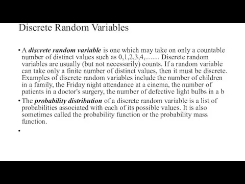
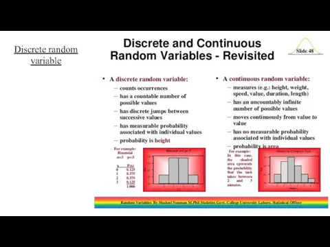
A discrete random variable is one which may take on only
a countable number of distinct values such as 0,1,2,3,4,........ Discrete random variables are usually (but not necessarily) counts. If a random variable can take only a finite number of distinct values, then it must be discrete. Examples of discrete random variables include the number of children in a family, the Friday night attendance at a cinema, the number of patients in a doctor's surgery, the number of defective light bulbs in a b
The probability distribution of a discrete random variable is a list of probabilities associated with each of its possible values. It is also sometimes called the probability function or the probability mass function.
Слайд 3
Слайд 4

Continuous Random Variables
A continuous random variable is one which takes an infinite number
of possible values. Continuous random variables are usually measurements. Examples include height, weight, the amount of sugar in an orange, the time required to run a mile.
A continuous random variable is not defined at specific values. Instead, it is defined over an interval of values, and is represented by the area under a curve (in advanced mathematics, this is known as an integral). The probability of observing any single value is equal to 0, since the number of values which may be assumed by the random variable is infinite.
Слайд 5
Suppose a random variable X may take all values over an interval of
real numbers. Then the probability that X is in the set of outcomes A, P(A), is defined to be the area above A and under a curve. The curve, which represents a function p(x), must satisfy the following:
1: The curve has no negative values (p(x) > 0 for all x)
2: The total area under the curve is equal to 1.
A curve meeting these requirements is known as a density curve.
Слайд 6
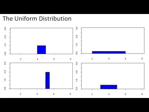
The Uniform Distribution
A random number generator acting over an interval of
numbers (a,b) has a continuous distribution. Since any interval of numbers of equal width has an equal probability of being observed, the curve describing the distribution is a rectangle, with constant height across the interval and 0 height elsewhere. Since the area under the curve must be equal to 1, the length of the interval determines the height of the curve.
The following graphs plot the density curves for random number generators over the intervals (4,5) (top left), (2,6) (top right), (5,5.5) (lower left), and (3,5) (lower right). The distributions corresponding to these curves are known as uniform distributions.
Слайд 7
Слайд 8

Consider the uniform random variable X defined on the interval (2,6). Since the
interval has width = 4, the curve has height = 0.25 over the interval and 0 elsewhere. The probability that X is less than or equal to 5 is the area between 2 and 5, or (5-2)*0.25 = 0.75. The probability that X is greater than 3 but less than 4 is the area between 3 and 4, (4-3)*0.25 = 0.25. To find that probability that X is less than 3 orgreater than 5, add the two probabilities:
P(X < 3 and X > 5) = P(X < 3) + P(X > 5) = (3-2)*0.25 + (6-5)*0.25 = 0.25 + 0.25 = 0.5.
The uniform distribution is often used to simulate data. Suppose you would like to simulate data for 10 rolls of a regular 6-sided die. Using the MINITAB "RAND" command with the "UNIF" subcommand generates 10 numbers in the interval (0,6):
Слайд 9

MTB > RAND 10 c2;
SUBC> unif 0 6.
Assign the discrete random
variable X to the values 1, 2, 3, 4, 5, or 6 as follows:
if 05, X=6.

 Таблица умножения двух
 Образование чисел из одного десятка и нескольких единиц. 1 класс
 Деление дробей. Урок 127
 Урок Сложение двузначных чисел в столбик, технология проблемного обучения
 Тест по логике № 1. Тема Понятие
 тренажёр по математике 1 класс
 Линейная функция и её график
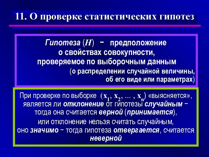 О проверке статистических гипотез
 Логарифмические уравнения. Уравнения, решаемые с использованием теорем о логарифмах
 Действия с геометрическими фигурами. Прототип задания B3, ЕГЭ
 Математика. 1 класс. Урок 86. Числа от 10 до 20 - Презентация
 Признаки параллельности прямых
 Симметрия
 Замечательные точки треугольника. Урок 1. Свойство биссектрисы угла
 Окружность. Радиус и диаметр окружности
 Комплексные числа. Основные понятия. Формы записи
 Решение задач. Урок математики для 4 класса
 Понятие формы. Многообразие форм окружающего мира
 Свойства параллелограмма
 Тела вращения. Цилиндр
 Слайд-шоу с методическим сопровождениемВ царстве геометрических фигур
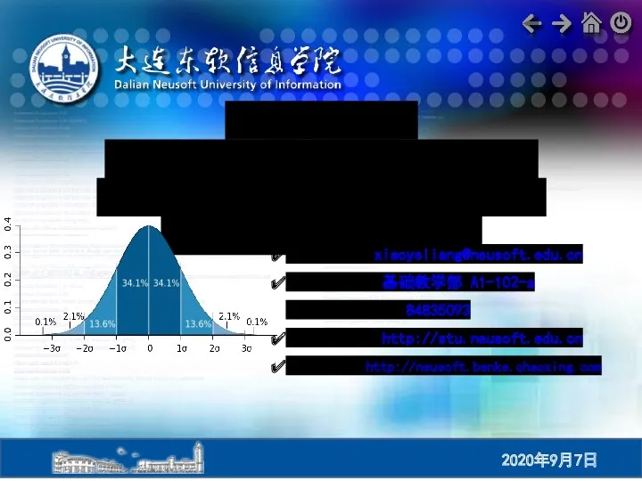 Теория вероятностей и математическая статистика
 Порядок действий в примерах со скобками. Презентация
 Комбинация призмы и цилиндра
 Разработка урока математики Вычитание числа 1 1 класс
 Тригонометрические формулы
 Тела вращения
 Презентация к уроку математики 2 кл. Угол. Виды углов и треугольников.