- Solution Methods Applied Computational Fluid Dynamics. Lecture 5

Содержание
- 2. Solution methods Focus on finite volume method. Background of finite volume method. Discretization example. General solution
- 3. Overview of numerical methods Many CFD techniques exist. The most common in commercially available CFD programs
- 4. Finite difference method (FDM) Historically, the oldest of the three. Techniques published as early as 1910
- 5. The domain is discretized into a series of grid points. A “structured” (ijk) mesh is required.
- 6. Earliest use was by Courant (1943) for solving a torsion problem. Clough (1960) gave the method
- 7. First well-documented use was by Evans and Harlow (1957) at Los Alamos and Gentry, Martin and
- 8. Divide the domain into control volumes. Integrate the differential equation over the control volume and apply
- 9. Cells and nodes Using finite volume method, the solution domain is subdivided into a finite number
- 10. The net flux through the control volume boundary is the sum of integrals over the four
- 11. Discretization example To illustrate how the conservation equations used in CFD can be discretized we will
- 12. Discretization example - continued The balance over the control volume is given by: This contains values
- 13. Discretization example - continued The simplest way to determine the values at the faces is by
- 14. Discretization example - continued Rearranging the previous equation results in: This equation can now be simplified
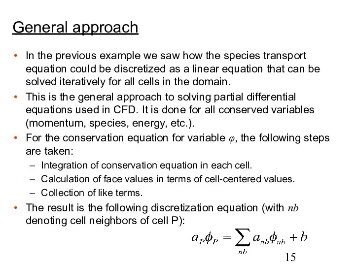
- 15. General approach In the previous example we saw how the species transport equation could be discretized
- 16. General approach - relaxation At each iteration, at each cell, a new value for variable φ
- 17. Underrelaxation recommendation Underrelaxation factors are there to suppress oscillations in the flow solution that result from
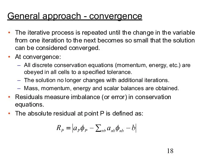
- 18. The iterative process is repeated until the change in the variable from one iteration to the
- 19. Residuals are usually scaled relative to the local value of the property φ in order to
- 20. Notes on convergence Always ensure proper convergence before using a solution: unconverged solutions can be misleading!!
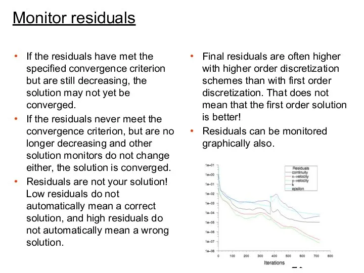
- 21. Monitor residuals If the residuals have met the specified convergence criterion but are still decreasing, the
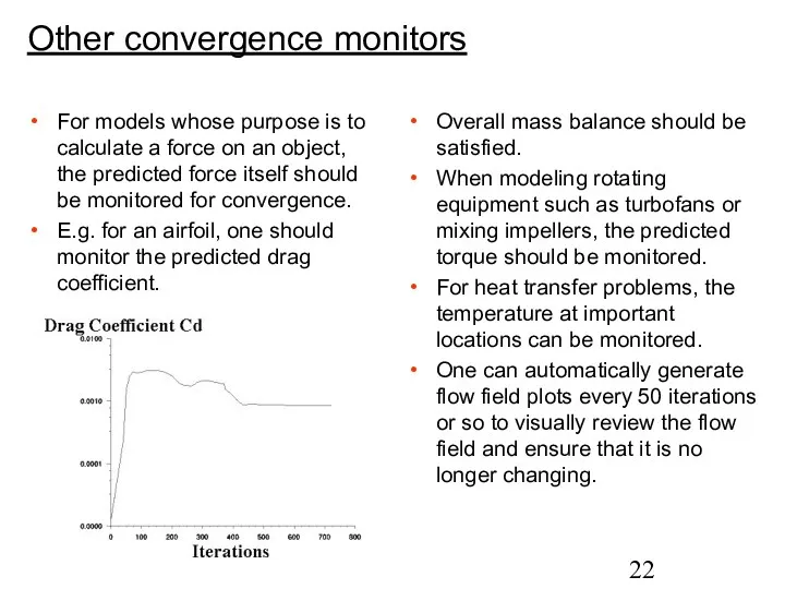
- 22. Other convergence monitors For models whose purpose is to calculate a force on an object, the
- 23. Face values of φ and ∂φ/∂x are found by making assumptions about variation of φ between
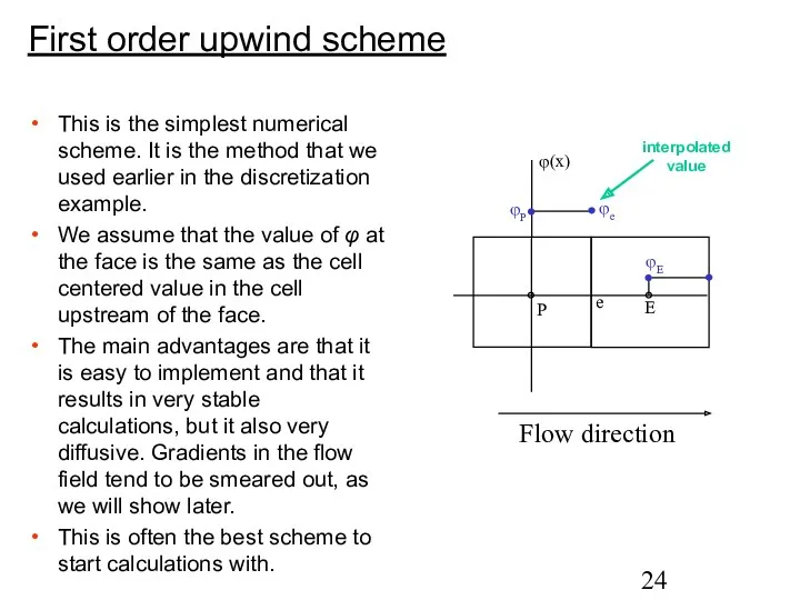
- 24. First order upwind scheme This is the simplest numerical scheme. It is the method that we
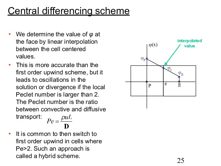
- 25. Central differencing scheme We determine the value of φ at the face by linear interpolation between
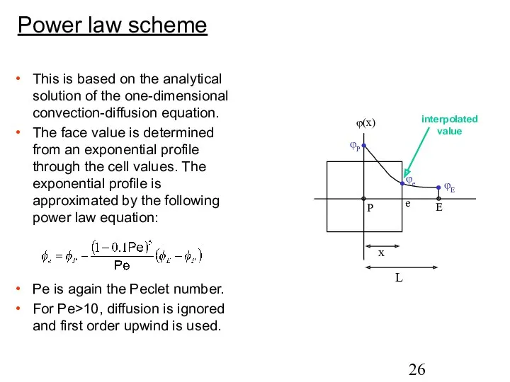
- 26. This is based on the analytical solution of the one-dimensional convection-diffusion equation. The face value is
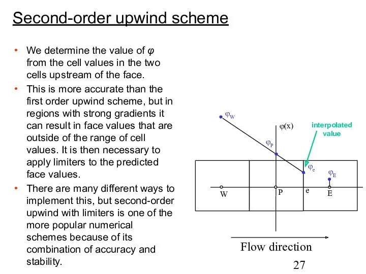
- 27. Second-order upwind scheme We determine the value of φ from the cell values in the two
- 28. QUICK scheme QUICK stands for Quadratic Upwind Interpolation for Convective Kinetics. A quadratic curve is fitted
- 29. Accuracy of numerical schemes Each of the previously discussed numerical schemes assumes some shape of the
- 30. Accuracy and false diffusion (1) False diffusion is numerically introduced diffusion and arises in convection dominated
- 31. Accuracy and false diffusion (2)
- 32. Properties of numerical schemes All numerical schemes must have the following properties: Conservativeness: global conservation of
- 33. Solution accuracy Higher order schemes will be more accurate. They will also be less stable and
- 34. Pressure We saw how convection-diffusion equations can be solved. Such equations are available for all variables,
- 35. Pressure - velocity coupling Pressure appears in all three momentum equations. The velocity field also has
- 36. Principle behind SIMPLE The principle behind SIMPLE is quite simple! It is based on the premise
- 37. Improvements on SIMPLE SIMPLE is the default algorithm in most commercial finite volume codes. Improved versions
- 38. Finite volume solution methods The finite volume solution method can either use a “segregated” or a
- 39. Segregated solution procedure
- 40. Coupled solution procedure When the coupled solver is used for steady state calculations it essentially employs
- 41. Unsteady solution procedure Same procedure for segregated and coupled solvers. The user has to specify a
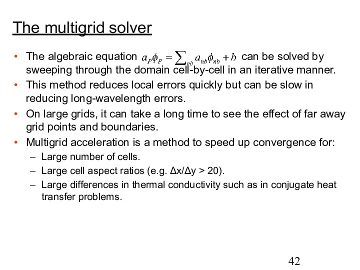
- 42. The multigrid solver The algebraic equation can be solved by sweeping through the domain cell-by-cell in
- 43. The multigrid solver uses a sequence of grids going from fine to coarse. The influence of
- 44. The solution on the coarser meshes is used as a starting point for solutions on the
- 46. Скачать презентацию
Solution methods
Focus on finite volume method.
Background of finite volume method.
Discretization example.
General
Solution methods
Focus on finite volume method.
Background of finite volume method.
Discretization example.
General
Overview of numerical methods
Many CFD techniques exist.
The most common in commercially
Overview of numerical methods
Many CFD techniques exist.
The most common in commercially
Finite difference method (FDM)
Historically, the oldest of the three.
Techniques published as
Finite difference method (FDM)
Historically, the oldest of the three.
Techniques published as
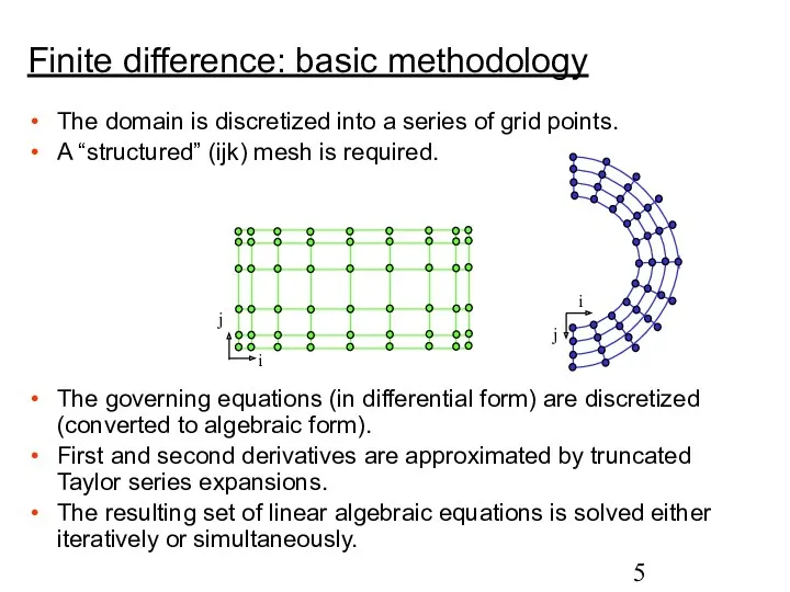
The domain is discretized into a series of grid points.
A “structured”
The domain is discretized into a series of grid points.
A “structured”
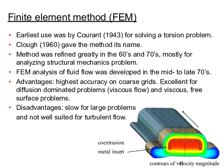
Earliest use was by Courant (1943) for solving a torsion problem.
Clough
Earliest use was by Courant (1943) for solving a torsion problem.
Clough
First well-documented use was by Evans and Harlow (1957) at Los
First well-documented use was by Evans and Harlow (1957) at Los
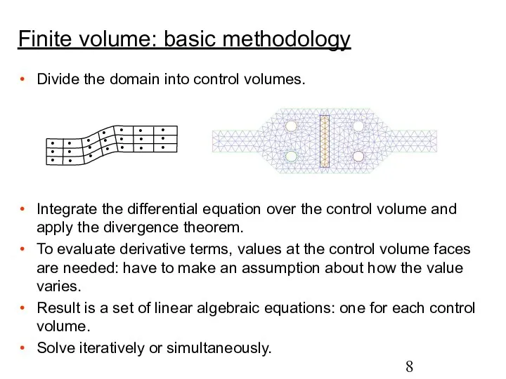
Divide the domain into control volumes.
Integrate the differential equation over
Divide the domain into control volumes.
Integrate the differential equation over
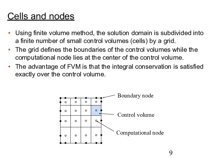
Cells and nodes
Using finite volume method, the solution domain is subdivided
Cells and nodes
Using finite volume method, the solution domain is subdivided

The net flux through the control volume boundary is the sum
The net flux through the control volume boundary is the sum
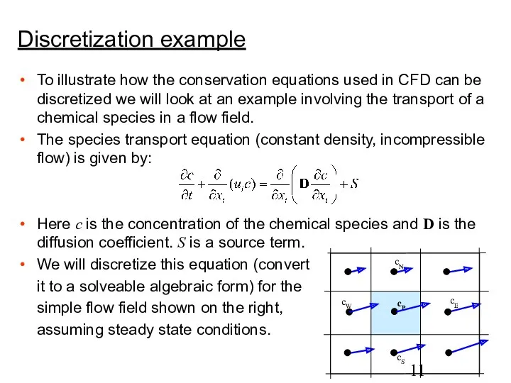
Discretization example
To illustrate how the conservation equations used in CFD can
Discretization example
To illustrate how the conservation equations used in CFD can
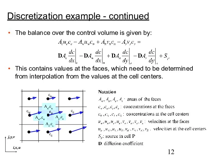
Discretization example - continued
The balance over the control volume is given
Discretization example - continued
The balance over the control volume is given
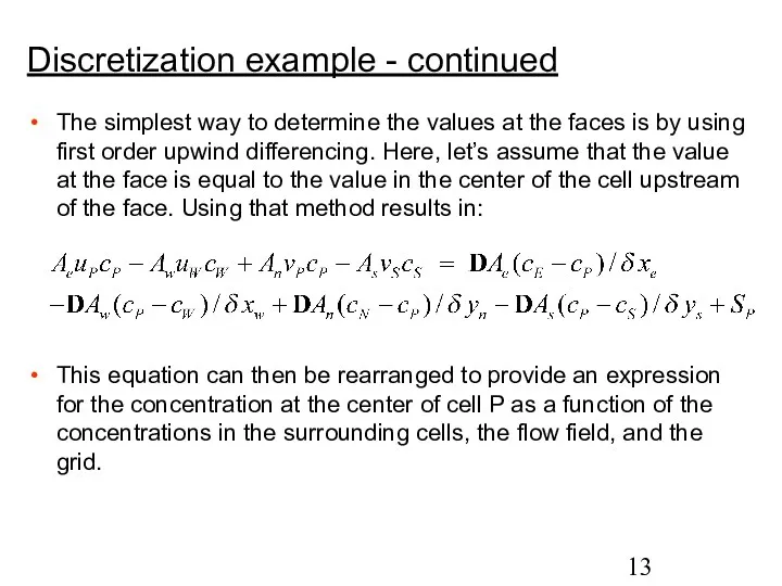
Discretization example - continued
The simplest way to determine the values at
Discretization example - continued
The simplest way to determine the values at
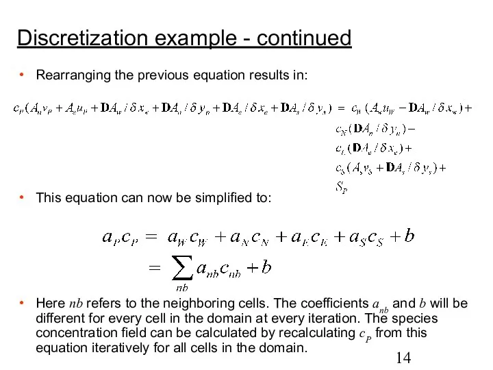
Discretization example - continued
Rearranging the previous equation results in:
This equation can
Discretization example - continued
Rearranging the previous equation results in:
This equation can
General approach
In the previous example we saw how the species transport
General approach
In the previous example we saw how the species transport

General approach - relaxation
At each iteration, at each cell, a new
General approach - relaxation
At each iteration, at each cell, a new
Underrelaxation recommendation
Underrelaxation factors are there to suppress oscillations in the flow
Underrelaxation recommendation
Underrelaxation factors are there to suppress oscillations in the flow
The iterative process is repeated until the change in the variable
The iterative process is repeated until the change in the variable
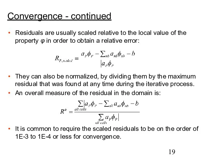
Residuals are usually scaled relative to the local value of the
Residuals are usually scaled relative to the local value of the
Notes on convergence
Always ensure proper convergence before using a solution: unconverged
Notes on convergence
Always ensure proper convergence before using a solution: unconverged
Monitor residuals
If the residuals have met the specified convergence criterion but
Monitor residuals
If the residuals have met the specified convergence criterion but
Other convergence monitors
For models whose purpose is to calculate a force
Other convergence monitors
For models whose purpose is to calculate a force
Face values of φ and ∂φ/∂x are found by making assumptions
Face values of φ and ∂φ/∂x are found by making assumptions
First order upwind scheme
This is the simplest numerical scheme. It is
First order upwind scheme
This is the simplest numerical scheme. It is
Central differencing scheme
We determine the value of φ at the face
Central differencing scheme
We determine the value of φ at the face
This is based on the analytical solution of the one-dimensional convection-diffusion
This is based on the analytical solution of the one-dimensional convection-diffusion
Second-order upwind scheme
We determine the value of φ from the cell
Second-order upwind scheme
We determine the value of φ from the cell
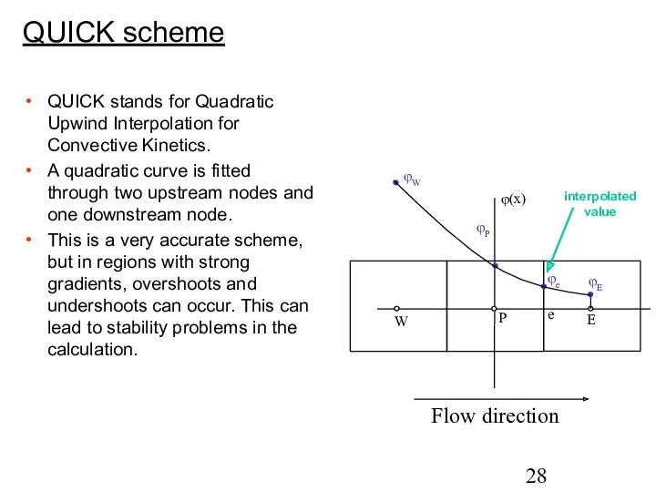
QUICK scheme
QUICK stands for Quadratic Upwind Interpolation for Convective Kinetics.
A quadratic
QUICK scheme
QUICK stands for Quadratic Upwind Interpolation for Convective Kinetics.
A quadratic
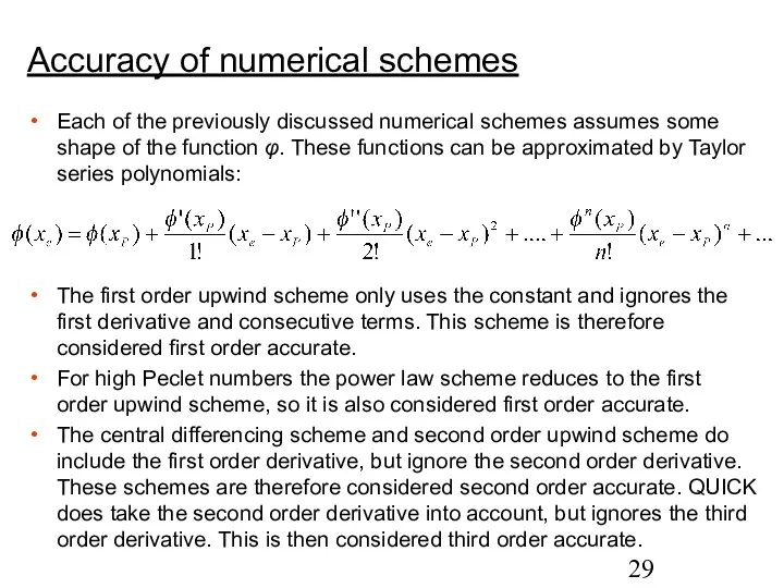
Accuracy of numerical schemes
Each of the previously discussed numerical schemes assumes
Accuracy of numerical schemes
Each of the previously discussed numerical schemes assumes
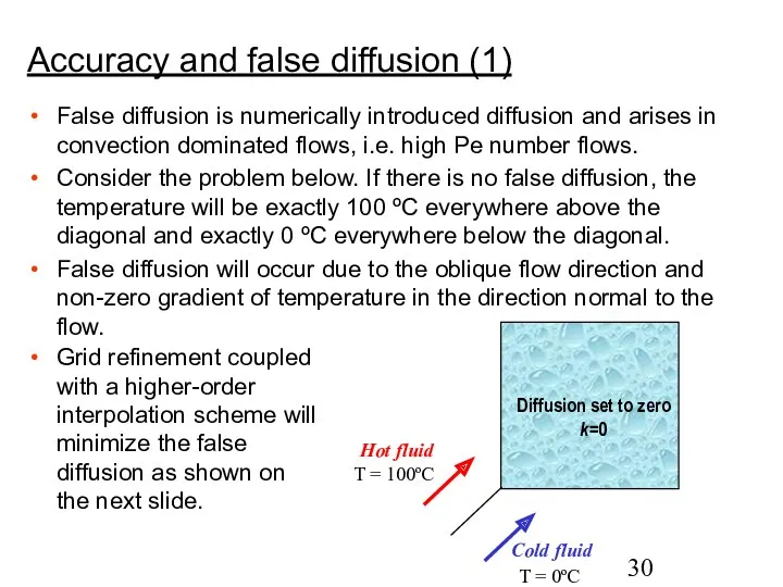
Accuracy and false diffusion (1)
False diffusion is numerically introduced diffusion and
Accuracy and false diffusion (1)
False diffusion is numerically introduced diffusion and
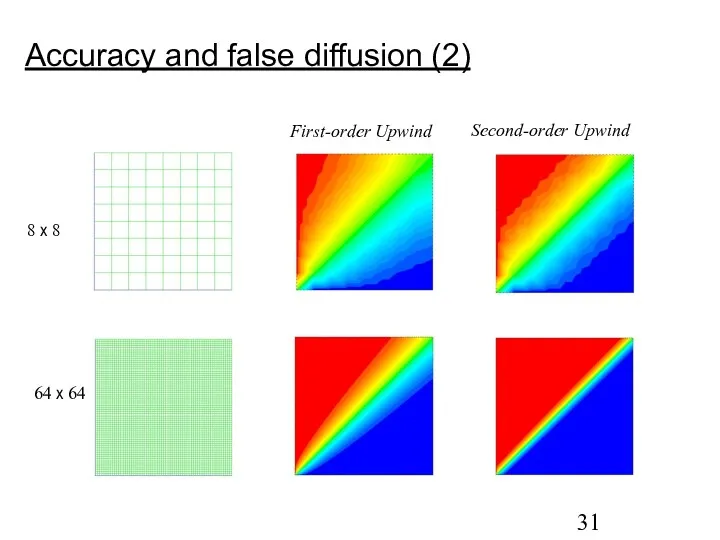
Accuracy and false diffusion (2)
Accuracy and false diffusion (2)
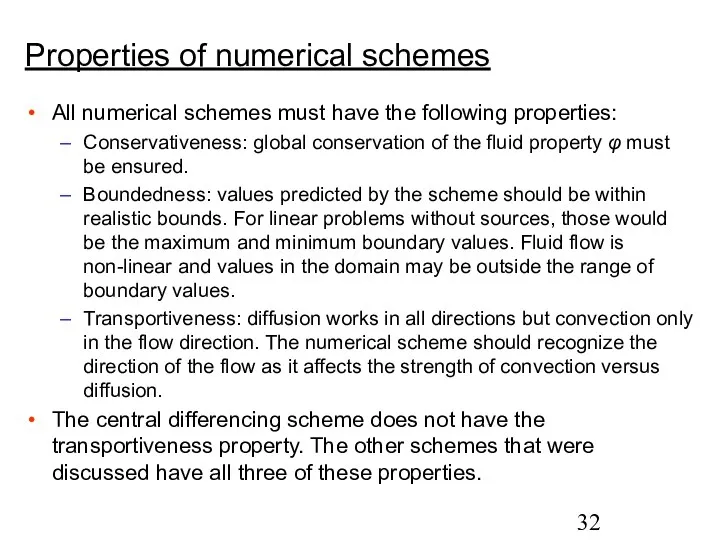
Properties of numerical schemes
All numerical schemes must have the following properties:
Conservativeness:
Properties of numerical schemes
All numerical schemes must have the following properties:
Conservativeness:
Solution accuracy
Higher order schemes will be more accurate. They will also
Solution accuracy
Higher order schemes will be more accurate. They will also
Pressure
We saw how convection-diffusion equations can be solved. Such equations are
Pressure
We saw how convection-diffusion equations can be solved. Such equations are
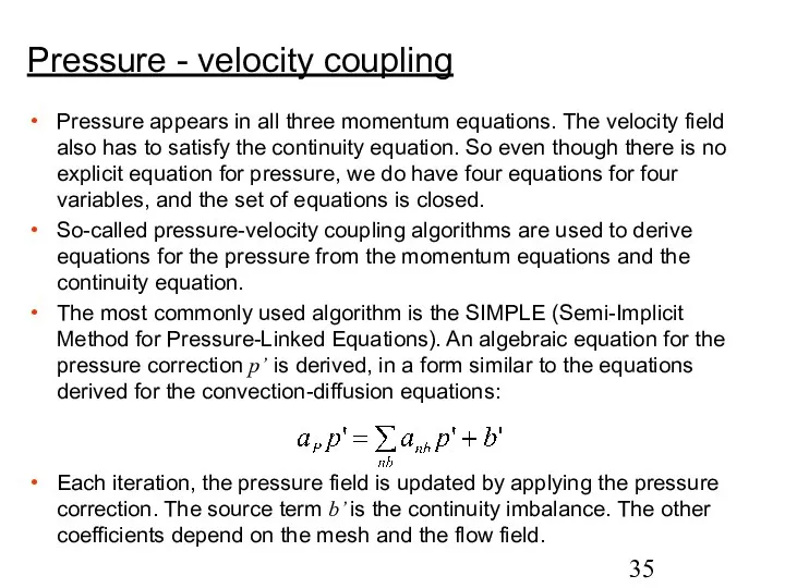
Pressure - velocity coupling
Pressure appears in all three momentum equations. The
Pressure - velocity coupling
Pressure appears in all three momentum equations. The
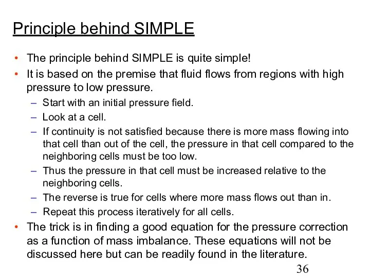
Principle behind SIMPLE
The principle behind SIMPLE is quite simple!
It is based
Principle behind SIMPLE
The principle behind SIMPLE is quite simple!
It is based
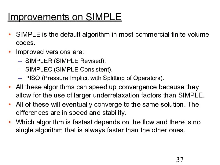
Improvements on SIMPLE
SIMPLE is the default algorithm in most commercial finite
Improvements on SIMPLE
SIMPLE is the default algorithm in most commercial finite
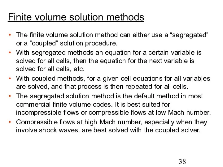
Finite volume solution methods
The finite volume solution method can either use
Finite volume solution methods
The finite volume solution method can either use

Segregated solution procedure
Segregated solution procedure
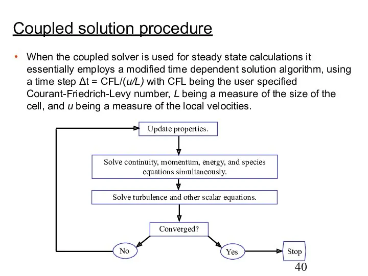
Coupled solution procedure
When the coupled solver is used for steady state
Coupled solution procedure
When the coupled solver is used for steady state
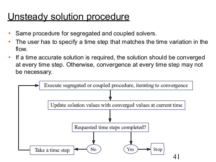
Unsteady solution procedure
Same procedure for segregated and coupled solvers.
The user has
Unsteady solution procedure
Same procedure for segregated and coupled solvers.
The user has
The multigrid solver
The algebraic equation can be solved by sweeping through
The multigrid solver
The algebraic equation can be solved by sweeping through
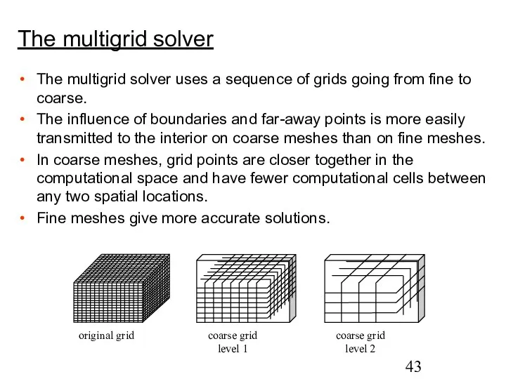
The multigrid solver uses a sequence of grids going from fine
The multigrid solver uses a sequence of grids going from fine
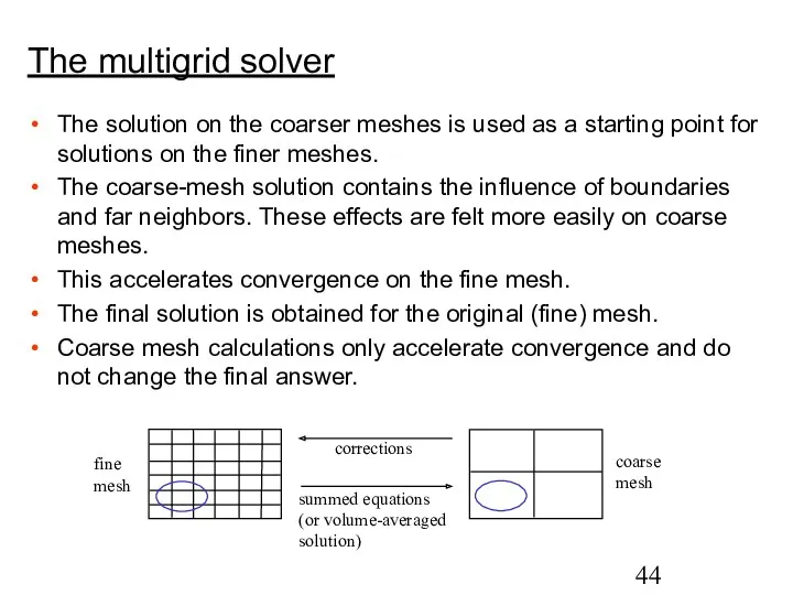
The solution on the coarser meshes is used as a starting
The solution on the coarser meshes is used as a starting
 Сложение и вычитание алгебраических дробей
 Разложение на простые множители
 Графики зависимости кинематических величин от времени при равномерном и равноускоренном движении
 Деление двузначного числа на однозначное.
 Применение производной к исследованию функции и построению графика функции
 Таблица умножения и деления на 3
 Площадь многоугольников
 Именованные числа.
 Задачи раскраски графов. Вершинная раскраска
 Сложение однозначных чисел с переходом через десяток, вида +2, +3
 Параллелограмм. Свойства параллелограмма
 Таблица сложения и вычитания в пределах 20 (КИМ 1 класс)
 Математика. 1 класс. Урок 7. Порядок
 Арифметическая прогрессия. Применение формул
 Урок математики в 3 классе по теме: Деление двузначного числа на однозначное
 Познавательно-игровой проект Применение игр и игровых упражнений с мячом в работе с детьми Диск
 Электронные обучающие игры для средней группы: Продолжи ряд, Сколько всего?
 Теорема синусов. Теорема косинусов
 Урок математики в 1 классе по теме Число пять. Цифра 5.
 Параллелограмм, трапеция, прямоугольник, квадрат, ромб. Обобщающий урок по геометрии для 8
 Повторение, обобщение и систематизация знаний. Степени с рациональным показателем
 Формулы - помощники для расчета расстояния, определения скорости движения, времени в пути
 Анализ временных рядов. (Тема 5)
 График линейной функции
 Санның логарифмі. Негізгі логарифмдік тепе-теңдік. Логарифмнің қасиеттері
 Пифагоров строй
 Прямая и обратная пропорциональные зависимости
 Ryspekov’s Fibonacci sequence formula