- The Simple Regression Model

Содержание
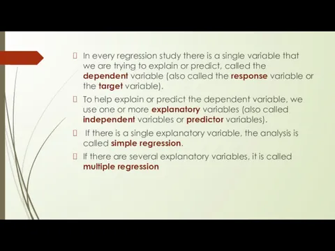
- 2. In every regression study there is a single variable that we are trying to explain or
- 3. The dependent (or response or target) variable is the single variable being explained by the regression.
- 4. A simple regression analysis includes a single explanatory variable, whereas multiple regression can include any number
- 5. SCATTERPLOTS: GRAPHING RELATIONSHIPS A good way to begin any regression analysis is to draw one or
- 6. Example Pharmex is a chain of drugstores that operates around the country. To see how effective
- 7. There are two variables: ■ Promote: Pharmex’s promotional expenditures as a percentage of those of the
- 8. Note that each of these variables is an index, not a dollar amount. For example, if
- 9. The company expects that there is a positive relationship between these two variables, so that regions
- 10. If it were perfect, a given value of Promote would prescribe the value of Sales exactly.
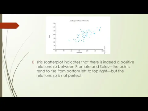
- 11. This scatterplot indicates that there is indeed a positive relationship between Promote and Sales—the points tend
- 12. Outliers Scatterplots are especially useful for identifying outliers, observations that lie outside the typical pattern of
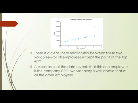
- 13. There is a clear linear relationship between these two variables—for all employees except the point at
- 14. An outlier is an observation that falls outside of the general pattern of the rest of
- 15. Although scatterplots are good for detecting outliers, they do not necessarily indicate what you ought to
- 16. First, the CEO’s salary is not determined in the same way as the salaries for typical
- 17. It is difficult to generalize about the treatment of outliers, but the following points are worth
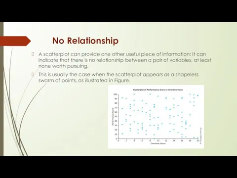
- 18. No Relationship A scatterplot can provide one other useful piece of information: It can indicate that
- 19. Here the variables are an employee performance score and the number of overtime hours worked in
- 20. CORRELATIONS: INDICATORS OF LINEAR RELATIONSHIPS Scatterplots provide graphical indications of relationships, whether they are linear, nonlinear,
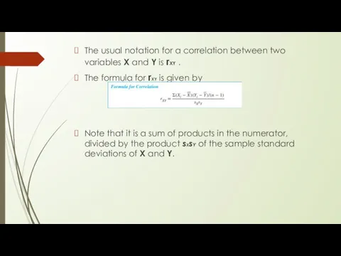
- 21. The usual notation for a correlation between two variables X and Y is rXY . The
- 22. The numerator of Equation is also a measure of association between two variables X and Y,
- 23. All correlations are between −1 and +1, inclusive. The sign of a correlation, plus or minus,
- 24. A correlation equal to 0 or near 0 indicates practically no linear relationship. A correlation with
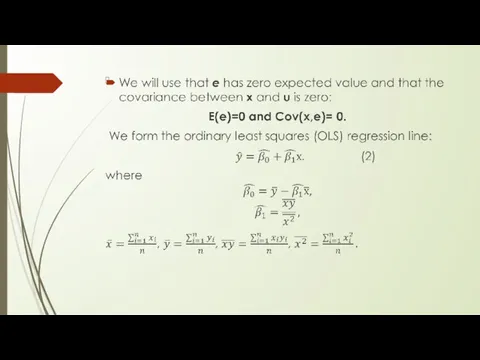
- 25. Least Squares Estimation The least squares line is the line that minimizes the sum of the
- 28. Thus, the change in y is simply β1 multiplied by the change in x. This means
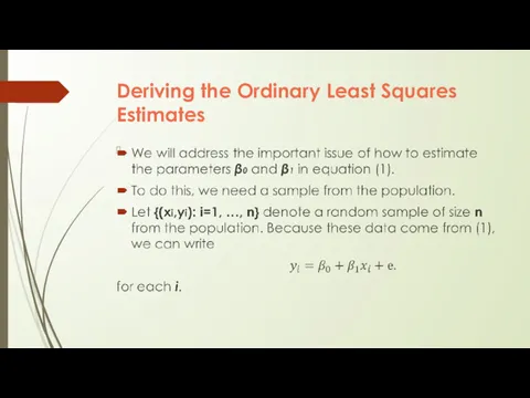
- 29. Deriving the Ordinary Least Squares Estimates
- 30. Here, ei is the error term for observation i because it contains all factors affecting yi
- 33. There are numerous residuals, it is useful to summarize them with a single numerical measure. This
- 36. Скачать презентацию
In every regression study there is a single variable that we
In every regression study there is a single variable that we
The dependent (or response or target) variable is the single variable
The dependent (or response or target) variable is the single variable
A simple regression analysis includes a single explanatory variable, whereas multiple
A simple regression analysis includes a single explanatory variable, whereas multiple
SCATTERPLOTS: GRAPHING RELATIONSHIPS
A good way to begin any regression analysis is
SCATTERPLOTS: GRAPHING RELATIONSHIPS
A good way to begin any regression analysis is

Example
Pharmex is a chain of drugstores that operates around the
Example
Pharmex is a chain of drugstores that operates around the

There are two variables:
■ Promote: Pharmex’s promotional expenditures as a
There are two variables:
■ Promote: Pharmex’s promotional expenditures as a
Note that each of these variables is an index, not a
Note that each of these variables is an index, not a
The company expects that there is a positive relationship between these
The company expects that there is a positive relationship between these

If it were perfect, a given value of Promote would prescribe
If it were perfect, a given value of Promote would prescribe
This scatterplot indicates that there is indeed a positive relationship between
This scatterplot indicates that there is indeed a positive relationship between

Outliers
Scatterplots are especially useful for identifying outliers, observations that lie outside
Outliers
Scatterplots are especially useful for identifying outliers, observations that lie outside
There is a clear linear relationship between these two variables—for all
There is a clear linear relationship between these two variables—for all
An outlier is an observation that falls outside of the general
An outlier is an observation that falls outside of the general

Although scatterplots are good for detecting outliers, they do not necessarily
Although scatterplots are good for detecting outliers, they do not necessarily

First, the CEO’s salary is not determined in the same way
First, the CEO’s salary is not determined in the same way

It is difficult to generalize about the treatment of outliers, but
It is difficult to generalize about the treatment of outliers, but
No Relationship
A scatterplot can provide one other useful piece of
No Relationship
A scatterplot can provide one other useful piece of
Here the variables are an employee performance score and the number
Here the variables are an employee performance score and the number
CORRELATIONS: INDICATORS OF LINEAR RELATIONSHIPS
Scatterplots provide graphical indications of relationships, whether
CORRELATIONS: INDICATORS OF LINEAR RELATIONSHIPS
Scatterplots provide graphical indications of relationships, whether
The usual notation for a correlation between two variables X and
The usual notation for a correlation between two variables X and
The numerator of Equation is also a measure of association between
The numerator of Equation is also a measure of association between
All correlations are between −1 and +1, inclusive.
The sign of
All correlations are between −1 and +1, inclusive.
The sign of
A correlation equal to 0 or near 0 indicates practically no
A correlation equal to 0 or near 0 indicates practically no
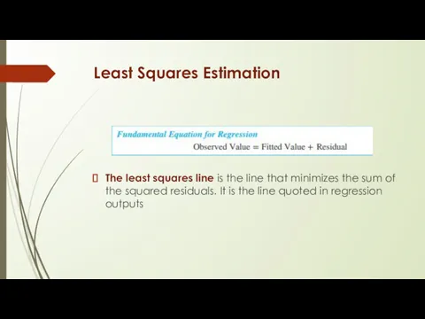
Least Squares Estimation
The least squares line is the line that
Least Squares Estimation
The least squares line is the line that
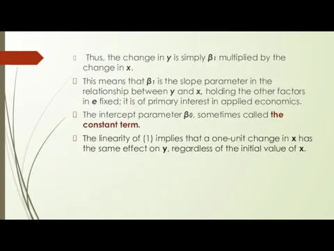
Thus, the change in y is simply β1 multiplied by the
Thus, the change in y is simply β1 multiplied by the
Deriving the Ordinary Least Squares Estimates
Deriving the Ordinary Least Squares Estimates
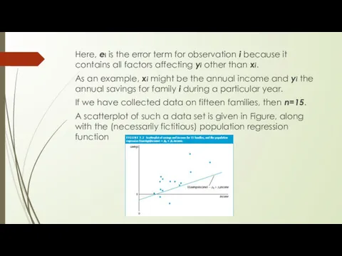
Here, ei is the error term for observation i because it

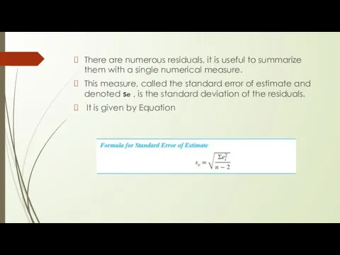
There are numerous residuals, it is useful to summarize them with
There are numerous residuals, it is useful to summarize them with

 математика Петерсон 2 класс Таблица умножения и деления с презентацией
 Прикладная статистика. Меры центральной тенденции. Меры разброса. Нормальное распределение
 Случайная величина (СВ) и закон ее распределения
 Геометрические преобразования пространства
 ИКТ при изучении темы Разные задачи на многогранники, цилиндр, конус и шар
 Взаємне розміщення площини і кулі у просторі
 Презентация Счёт в пределах 1000
 Формы организации учебной деятельности учащихся на уроке математики
 Обыкновенные дроби. Деление дробей
 Методическое пособие по математике Состав числа 6
 Математический турнир знатоков, 8 класс
 Повторение теоретического материала по геометрии 7 класс
 Математический анализ
 Параллелепипед. Грани, ребра, диагональ параллелепипеда
 Сумма углов треугольника. Тренировочные упражнения
 Матрицы. Метод Гаусса. Формулы Крамера
 Некоторые следствия из аксиом
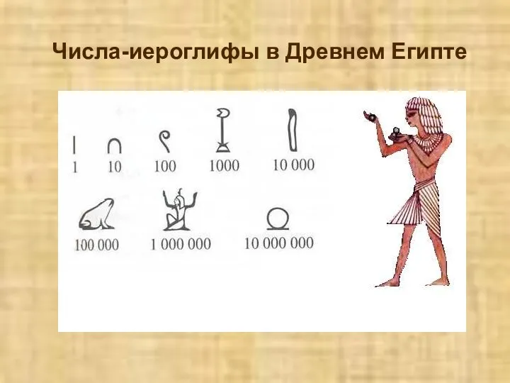 Числа-иероглифы в Древнем Египте
 Скалярное произведение векторов. Вычисление углов между прямыми
 Неравенство треугольника
 Тренажёр по математике (2 класс)
 Метод координат
 Формула корней квадратного уравнения
 Прямая и обратная пропорциональные зависимости
 Арифметический квадратный корень
 История комплексных чисел от Кардано до Гамильтона
 Внеурочное мероприятие по математике В гостях у Квадратика в специальном классе школы 8 вида
 Деление с остатком