- Introduction to statistics

Содержание
- 2. The structure of presentation: A lot of definitions Main concepts of statistics Be ready to learn
- 3. Variables A variable is a characteristic or condition that can change or take on different values.
- 4. Population The entire group of individuals is called the population. For example, a researcher may be
- 5. Sample Usually populations are so large that a researcher cannot examine the entire group. Therefore, a
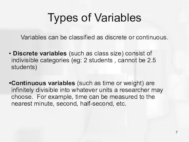
- 7. Types of Variables Variables can be classified as discrete or continuous. Discrete variables (such as class
- 8. Measuring Variables To establish relationships between variables, researchers must observe the variables and record their observations.
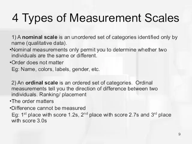
- 9. 4 Types of Measurement Scales 1) A nominal scale is an unordered set of categories identified
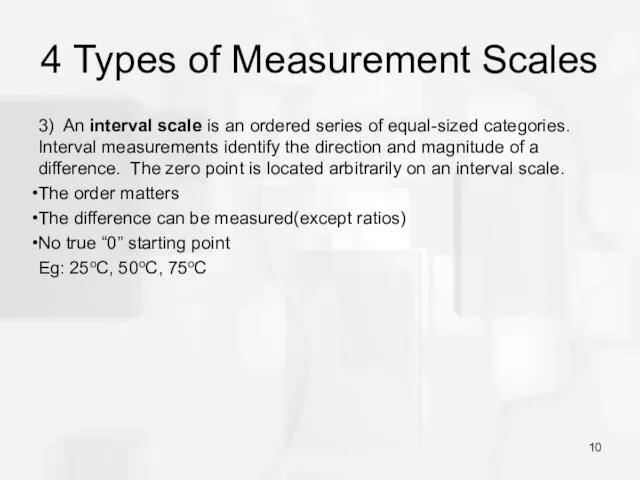
- 10. 4 Types of Measurement Scales 3) An interval scale is an ordered series of equal-sized categories.
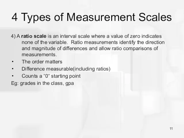
- 11. 4 Types of Measurement Scales 4) A ratio scale is an interval scale where a value
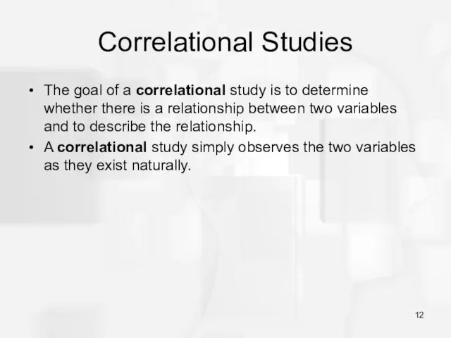
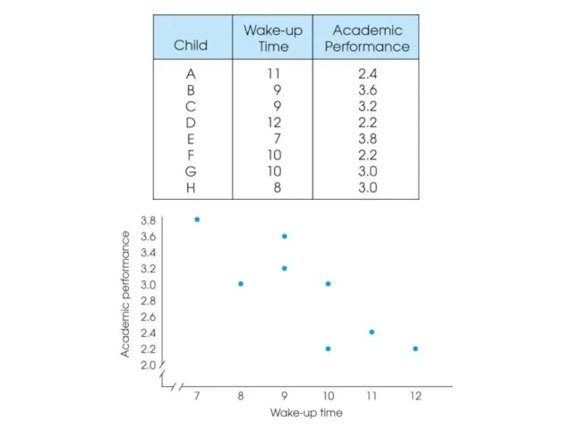
- 12. Correlational Studies The goal of a correlational study is to determine whether there is a relationship
- 14. Experiments The goal of an experiment is to demonstrate a cause-and-effect relationship between two variables; that
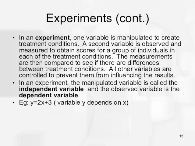
- 15. Experiments (cont.) In an experiment, one variable is manipulated to create treatment conditions. A second variable
- 17. Data The measurements obtained in a research study are called the data. The goal of statistics
- 18. Descriptive Statistics Descriptive statistics are methods for organizing and summarizing data. For example, tables or graphs
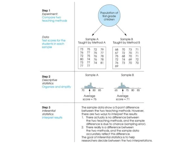
- 19. Inferential Statistics Inferential statistics are methods for using sample data to make general conclusions (inferences) about
- 20. Descriptive Organizing and summarizing data using numbers and graphs Data summary: Bar graphs, histograms, Pie Charts,
- 21. Sampling Error The discrepancy between a sample statistic and its population parameter is called sampling error.
- 22. Ungrouped Data vs Grouped Data Ungrouped Data – is a data with an individual value. Grouped
- 23. Frequency distribution. Ungrouped Data Eg: 2,3,3,5,7,7,7,7,8 ? ungrouped data ? Frequency table
- 24. Frequency distribution. Grouped data Eg. In the survey it has been observed that, there are 10
- 25. The Mean The mean for ungrouped data, also known as the arithmetic average, is found by
- 26. Taking a previous example. Eg: 2,3,3,5,7,7,7,7,8 ? Frequency table sample mean =? sample mean =sum/ n
- 27. The Median The median is the middle term in a data set. There are two possibilities
- 28. The Mode The value that occurs most often in a data set is called the mode.
- 29. Measures of dispersion for ungrouped data Consider the following 2 examples: Each of these samples has
- 30. Measures of dispersion The measures that help us to know about the spread of data set
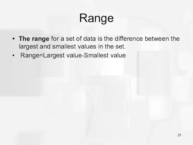
- 31. Range The range for a set of data is the difference between the largest and smallest
- 32. The mean absolute deviation The mean absolute deviation is defined exactly as the words indicate. The
- 33. Mean Absolute deviation (MAD)
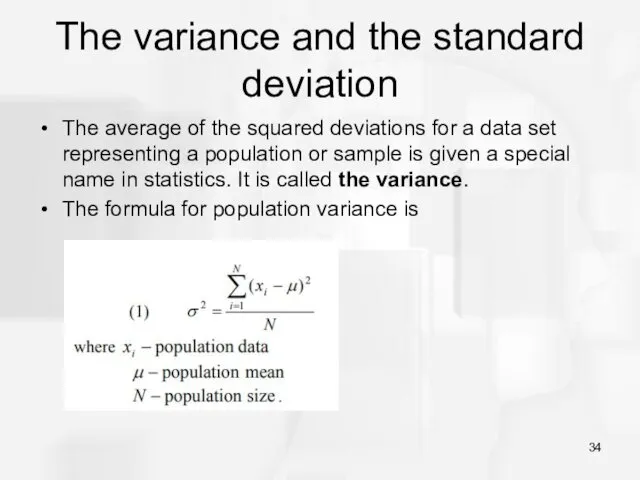
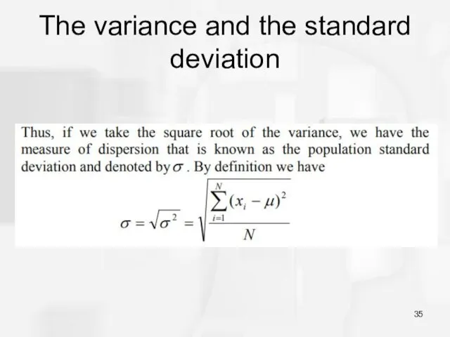
- 34. The variance and the standard deviation The average of the squared deviations for a data set
- 35. The variance and the standard deviation
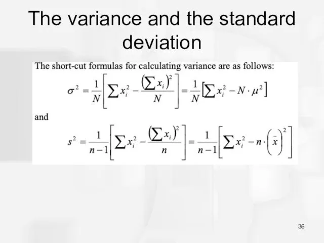
- 36. The variance and the standard deviation
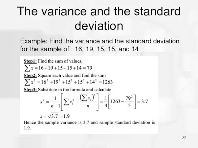
- 37. The variance and the standard deviation Example: Find the variance and the standard deviation for the
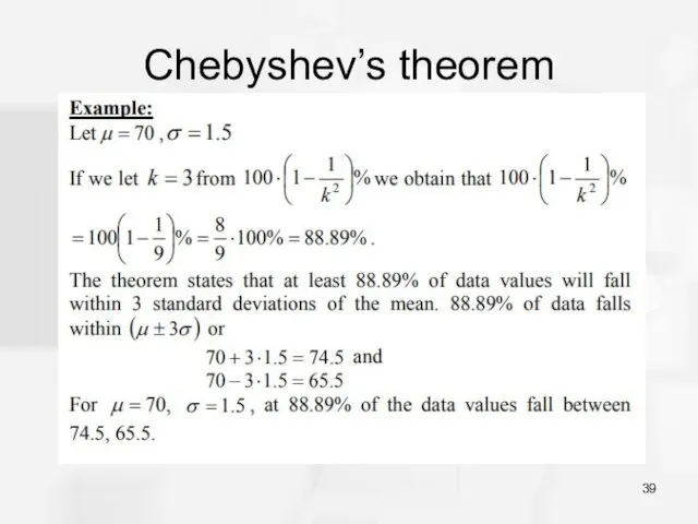
- 38. Chebyshev’s theorem
- 39. Chebyshev’s theorem
- 40. The interquartile range
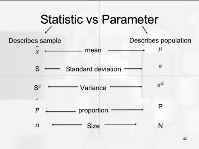
- 41. Small revision
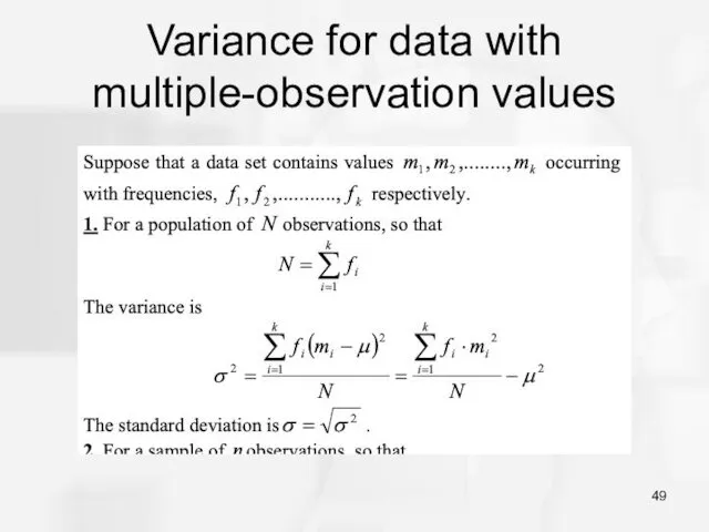
- 43. Mean for data with multiple-observation values For Population: Mean:
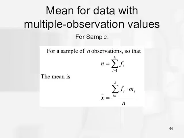
- 44. Mean for data with multiple-observation values For Sample:
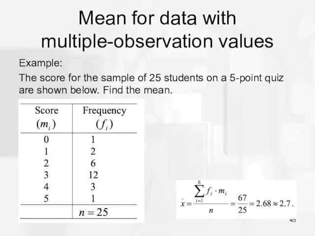
- 45. Mean for data with multiple-observation values Example: The score for the sample of 25 students on
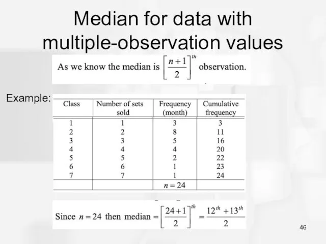
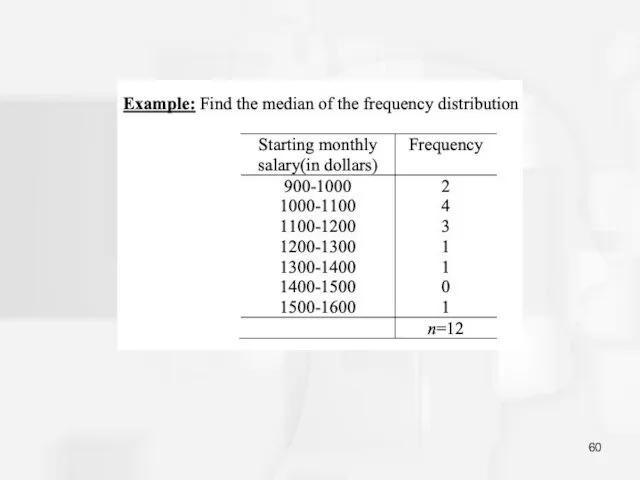
- 46. Median for data with multiple-observation values Example:
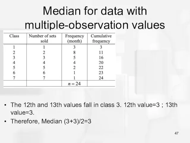
- 47. Median for data with multiple-observation values The 12th and 13th values fall in class 3. 12th
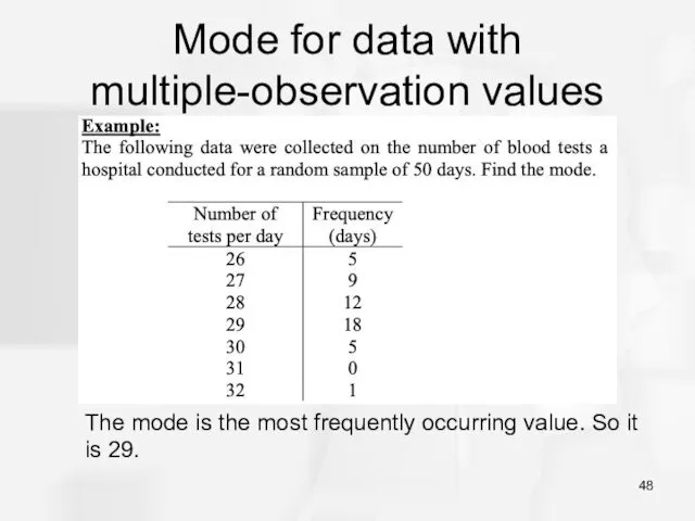
- 48. Mode for data with multiple-observation values The mode is the most frequently occurring value. So it
- 49. Variance for data with multiple-observation values
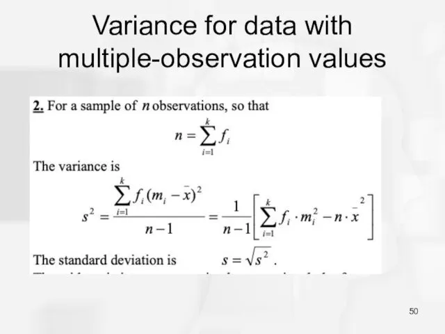
- 50. Variance for data with multiple-observation values
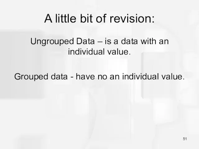
- 51. A little bit of revision: Ungrouped Data – is a data with an individual value. Grouped
- 52. Frequency distribution. Grouped data Eg. In the survey it has been observed that, there are 10
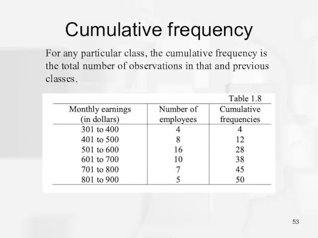
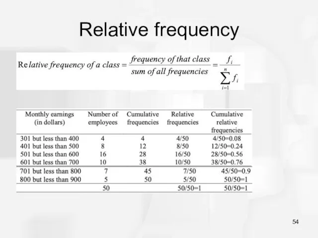
- 53. Cumulative frequency For any particular class, the cumulative frequency is the total number of observations in
- 54. Relative frequency
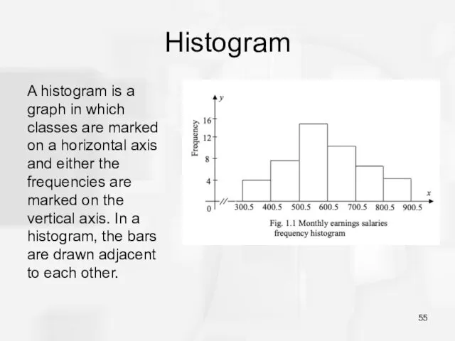
- 55. Histogram A histogram is a graph in which classes are marked on a horizontal axis and
- 56. Mean for grouped data
- 58. Solution:
- 59. The Median for grouped data
- 61. Find median Form cumulative frequency 3. Use formula
- 62. Median =12/2=6 Cumulative frequency: Substitute into the formula:
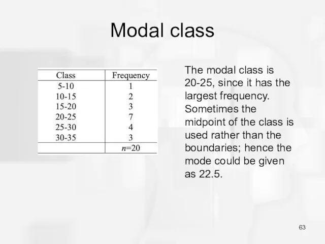
- 63. Modal class The modal class is 20-25, since it has the largest frequency. Sometimes the midpoint
- 64. Variance and standard deviation for grouped data
- 66. Скачать презентацию
The structure of presentation:
A lot of definitions
Main concepts of statistics
Be ready
The structure of presentation:
A lot of definitions
Main concepts of statistics
Be ready
Variables
A variable is a characteristic or condition that can change or
Variables
A variable is a characteristic or condition that can change or
Population
The entire group of individuals is called the population.
For example,
Population
The entire group of individuals is called the population.
For example,
Sample
Usually populations are so large that a researcher cannot examine the
Sample
Usually populations are so large that a researcher cannot examine the

Types of Variables
Variables can be classified as discrete or continuous.
Discrete variables
Types of Variables
Variables can be classified as discrete or continuous.
Discrete variables
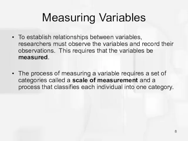
Measuring Variables
To establish relationships between variables, researchers must observe the variables
Measuring Variables
To establish relationships between variables, researchers must observe the variables
4 Types of Measurement Scales
1) A nominal scale is an unordered
4 Types of Measurement Scales
1) A nominal scale is an unordered
4 Types of Measurement Scales
3) An interval scale is an ordered
4 Types of Measurement Scales
3) An interval scale is an ordered
4 Types of Measurement Scales
4) A ratio scale is an interval
4 Types of Measurement Scales
4) A ratio scale is an interval
Correlational Studies
The goal of a correlational study is to determine whether
Correlational Studies
The goal of a correlational study is to determine whether
Experiments
The goal of an experiment is to demonstrate a cause-and-effect relationship
Experiments
The goal of an experiment is to demonstrate a cause-and-effect relationship
Experiments (cont.)
In an experiment, one variable is manipulated to create treatment
Experiments (cont.)
In an experiment, one variable is manipulated to create treatment
Data
The measurements obtained in a research study are called the data.
Data
The measurements obtained in a research study are called the data.
Descriptive Statistics
Descriptive statistics are methods for organizing and summarizing data.
For
Descriptive Statistics
Descriptive statistics are methods for organizing and summarizing data.
For
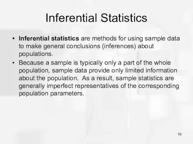
Inferential Statistics
Inferential statistics are methods for using sample data to make
Inferential Statistics
Inferential statistics are methods for using sample data to make
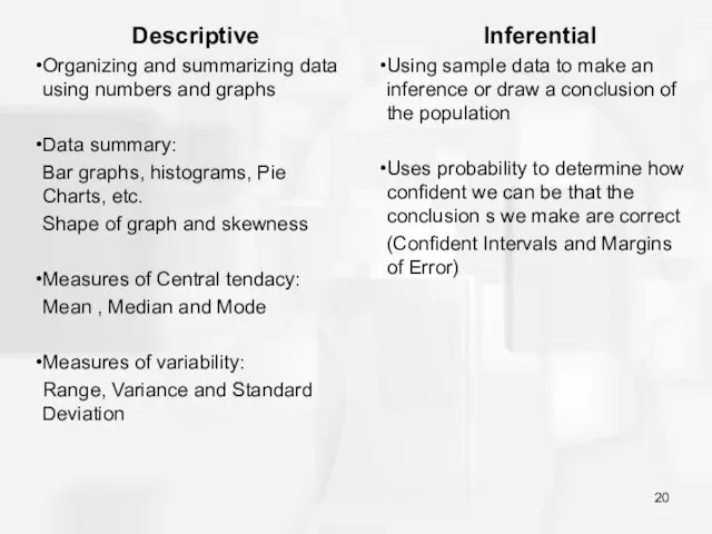
Descriptive
Organizing and summarizing data using numbers and graphs
Data summary:
Bar graphs,
Descriptive
Organizing and summarizing data using numbers and graphs
Data summary:
Bar graphs,
Sampling Error
The discrepancy between a sample statistic and its population parameter
Sampling Error
The discrepancy between a sample statistic and its population parameter
Ungrouped Data vs Grouped Data
Ungrouped Data – is a data with
Ungrouped Data vs Grouped Data
Ungrouped Data – is a data with
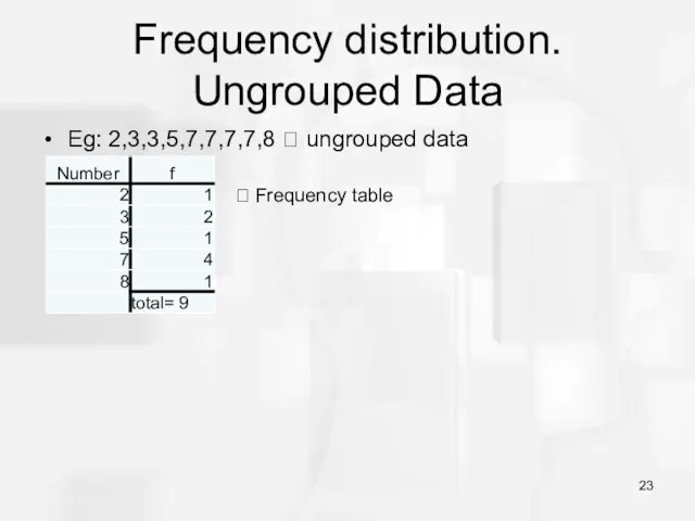
Frequency distribution. Ungrouped Data
Eg: 2,3,3,5,7,7,7,7,8 ? ungrouped data
? Frequency table
Frequency distribution. Ungrouped Data
Eg: 2,3,3,5,7,7,7,7,8 ? ungrouped data
? Frequency table
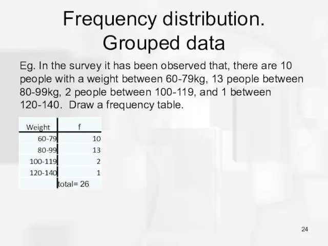
Frequency distribution.
Grouped data
Eg. In the survey it has been observed
Frequency distribution.
Grouped data
Eg. In the survey it has been observed
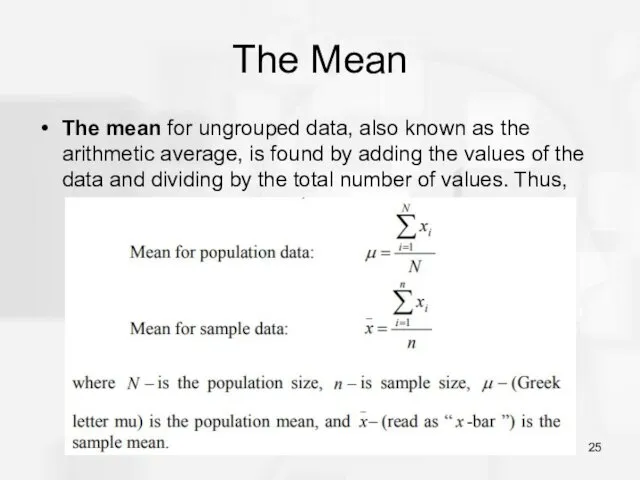
The Mean
The mean for ungrouped data, also known as the arithmetic
The Mean
The mean for ungrouped data, also known as the arithmetic
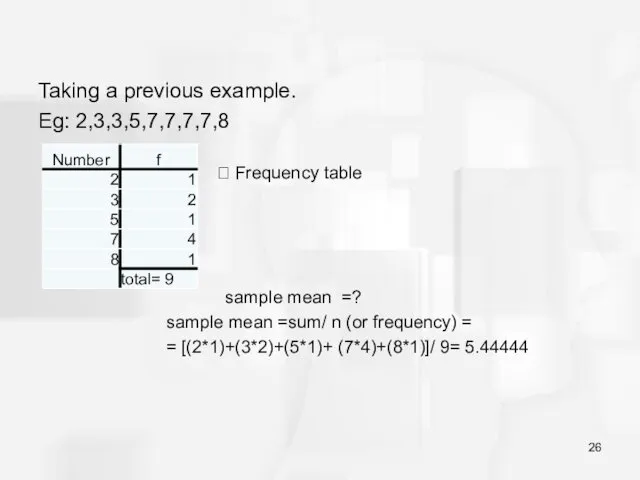
Taking a previous example.
Eg: 2,3,3,5,7,7,7,7,8
? Frequency table
sample mean =?
sample mean
Taking a previous example.
Eg: 2,3,3,5,7,7,7,7,8
? Frequency table
sample mean =?
sample mean
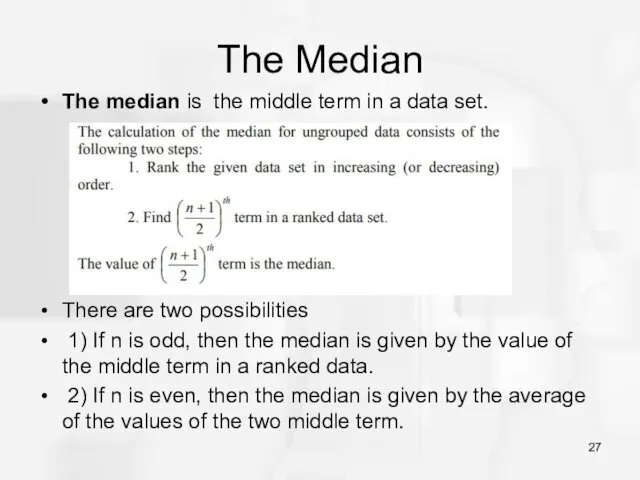
The Median
The median is the middle term in a data set.
There
The Median
The median is the middle term in a data set.
There
The Mode
The value that occurs most often in a data set
The Mode
The value that occurs most often in a data set
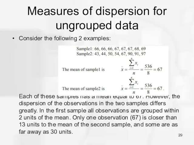
Measures of dispersion for ungrouped data
Consider the following 2 examples:
Each of
Measures of dispersion for ungrouped data
Consider the following 2 examples:
Each of
Measures of dispersion
The measures that help us to know about the
Measures of dispersion
The measures that help us to know about the
Range
The range for a set of data is the difference between
Range
The range for a set of data is the difference between
The mean absolute deviation
The mean absolute deviation is defined exactly as
The mean absolute deviation
The mean absolute deviation is defined exactly as
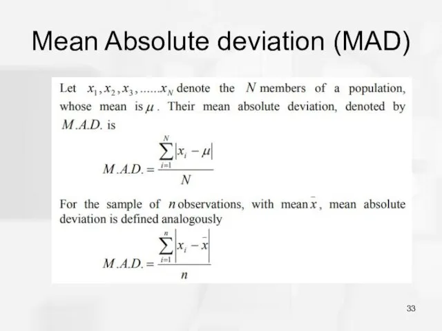
Mean Absolute deviation (MAD)
Mean Absolute deviation (MAD)
The variance and the standard deviation
The average of the squared deviations
The variance and the standard deviation
The average of the squared deviations
The variance and the standard deviation
The variance and the standard deviation
The variance and the standard deviation
The variance and the standard deviation
The variance and the standard deviation
Example: Find the variance and the
The variance and the standard deviation
Example: Find the variance and the

Chebyshev’s theorem
Chebyshev’s theorem
Chebyshev’s theorem
Chebyshev’s theorem
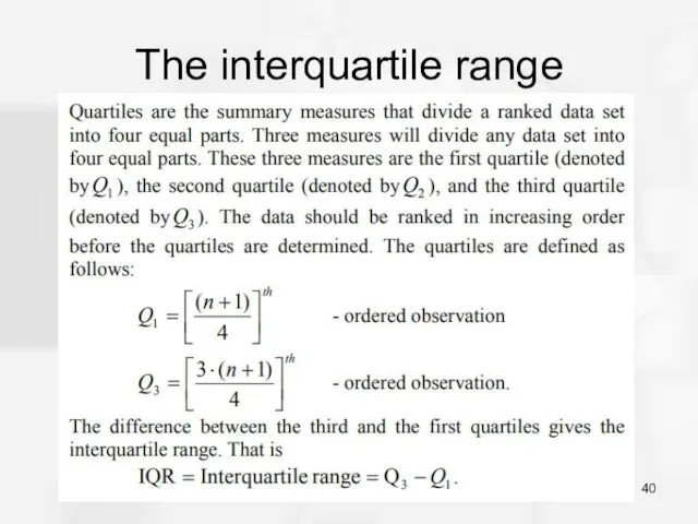
The interquartile range
The interquartile range

Small revision
Small revision
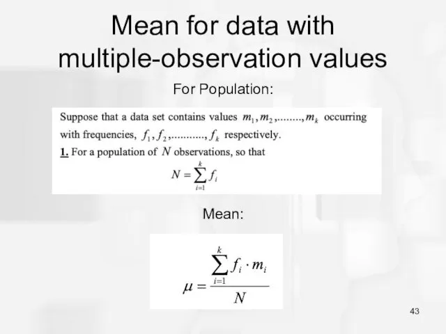
Mean for data with multiple-observation values
For Population:
Mean:
Mean for data with multiple-observation values
For Population:
Mean:
Mean for data with multiple-observation values
For Sample:
Mean for data with multiple-observation values
For Sample:
Mean for data with multiple-observation values
Example:
The score for the sample of
Mean for data with multiple-observation values
Example:
The score for the sample of
Median for data with multiple-observation values
Example:
Median for data with multiple-observation values
Example:
Median for data with multiple-observation values
The 12th and 13th values
Median for data with multiple-observation values
The 12th and 13th values
Mode for data with multiple-observation values
The mode is the most
Mode for data with multiple-observation values
The mode is the most
Variance for data with multiple-observation values
Variance for data with multiple-observation values
Variance for data with multiple-observation values
Variance for data with multiple-observation values
A little bit of revision:
Ungrouped Data – is a data with
A little bit of revision:
Ungrouped Data – is a data with

Frequency distribution.
Grouped data
Eg. In the survey it has been observed
Frequency distribution.
Grouped data
Eg. In the survey it has been observed
Cumulative frequency
For any particular class, the cumulative frequency is the total
Cumulative frequency
For any particular class, the cumulative frequency is the total
Relative frequency
Relative frequency
Histogram
A histogram is a graph in which classes are marked on
Histogram
A histogram is a graph in which classes are marked on
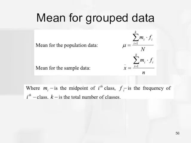
Mean for grouped data
Mean for grouped data
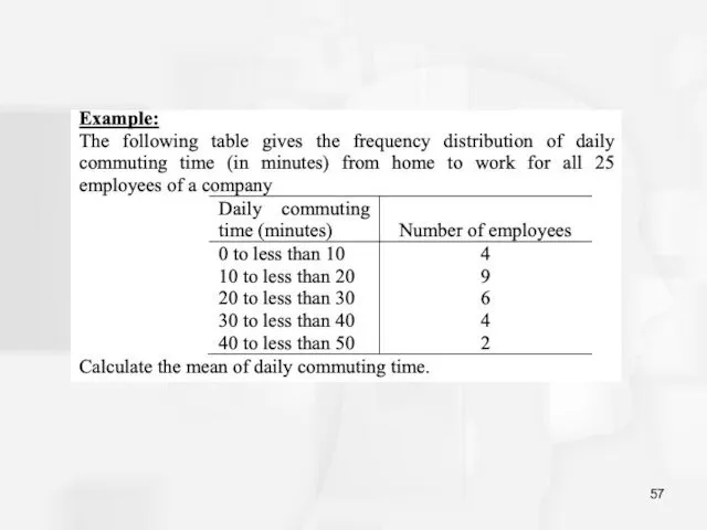
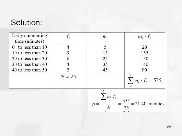
Solution:
Solution:
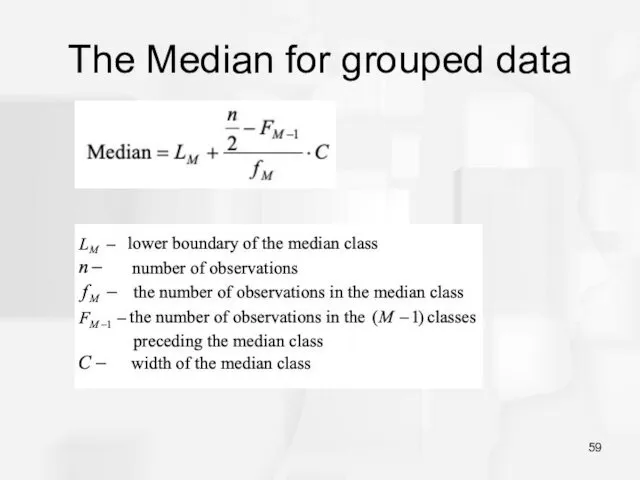
The Median for grouped data
The Median for grouped data
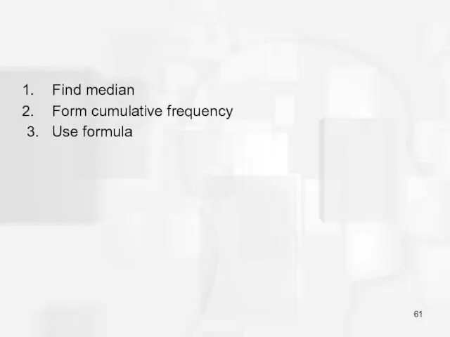
Find median
Form cumulative frequency
3. Use formula
Find median
Form cumulative frequency
3. Use formula
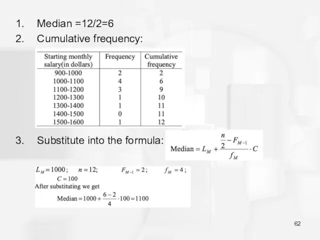
Median =12/2=6
Cumulative frequency:
Substitute into the formula:
Median =12/2=6
Cumulative frequency:
Substitute into the formula:
Modal class
The modal class is 20-25, since it has the
Modal class
The modal class is 20-25, since it has the
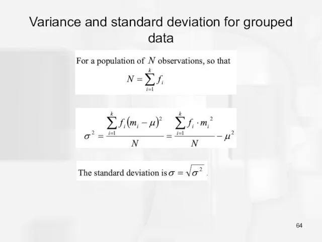
Variance and standard deviation for grouped data
Variance and standard deviation for grouped data
 Презентация Знакомство с решётками нашего города
 Снежинки
 Краткий тезаурус по ВВЭР-1200
 Кто как к зиме приготовился
 Имя прилагательное. Изменение по родам и числам
 Презентация : коротко об Олимпиаде в Москве в 1980 г.
 Пресуппозиции в тексте. Понятие пресупозиции. Характер связи пресуппозиции с контекстом. Пресуппозиция в тексте
 Алгоритм дизайна
 Макет бізнес-плану
 Репродукции для тестирования по истории изобразительного искусства в 3 классе ДХШ. Западноевропейское искусство
 Выпуклый анализ. Выпуклые множества. Лекция 8
 Слух у человека
 Деление, сложение, умножение
 Организация сюжетно - ролевых игр по ПДД
 Травматологиядағы шұғыл жағдайлар. Бассүйек-мидың жабық жарақаты
 Поделка Снеговик.
 Задача стационарной теплопередачи на примере полуограниченной пластины и длинного цилиндра
 Занятие 4: Начало работы с Arduino UNO R3
 Римское войско
 Теплоснабжение и отопление
 Твердотельная электроника. Полупроводниковые диоды
 Бермудский треугольник. 7 класс
 Корригирующие операции при деформации суставов
 классный час 4 ноября - день народного единства
 Кетоацидоздық кома
 Организация воинского учета. Первоначальная постановка граждан на воинский учет
 Методика применения интерактивной доски на уроке химии в 8 классе в теме Кислоты
 20231204_prezentatsiya_k_proektu_vliyanie_yaichnoy_skorlupy_na_plodorodie_pochvy