- Karnaugh maps

Содержание
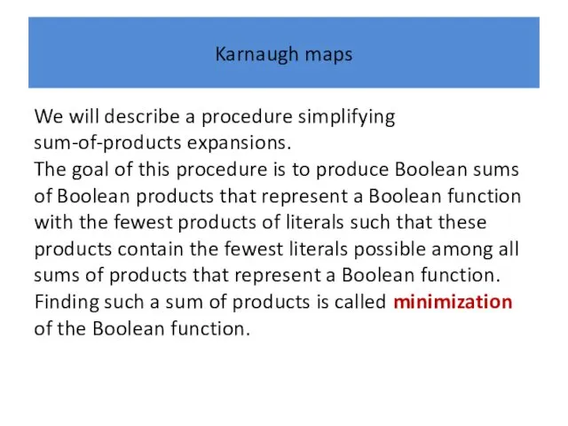
- 2. Karnaugh maps We will describe a procedure simplifying sum-of-products expansions. The goal of this procedure is
- 3. Karnaugh maps The procedure we will introduce, known as Karnaugh maps (or K-maps), was designed in
- 4. Karnaugh maps To reduce the number of terms in a Boolean expression it is necessary to
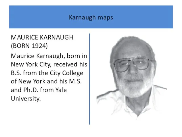
- 5. Karnaugh maps MAURICE KARNAUGH (BORN 1924) Maurice Karnaugh, born in New York City, received his B.S.
- 6. Karnaugh maps He was a member of the technical staff at Bell Laboratories from 1952 until
- 7. Karnaugh maps In 1970 he joined IBM as a member of the research staff.
- 8. Karnaugh maps Karnaugh has made fundamental contributions to the application of digital techniques in both computing
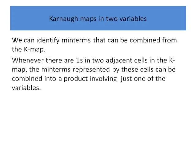
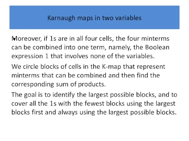
- 9. Karnaugh maps K-maps give us a visual method for simplifying sum-of-products expansions; they are not suited
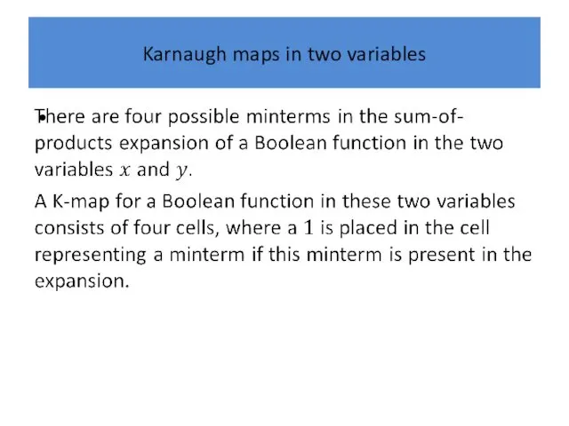
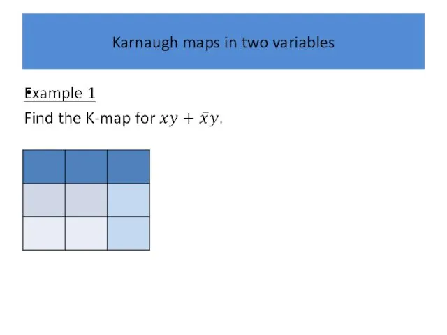
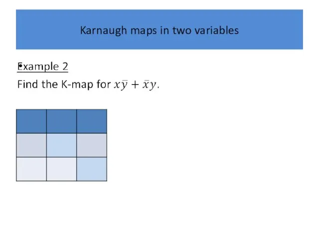
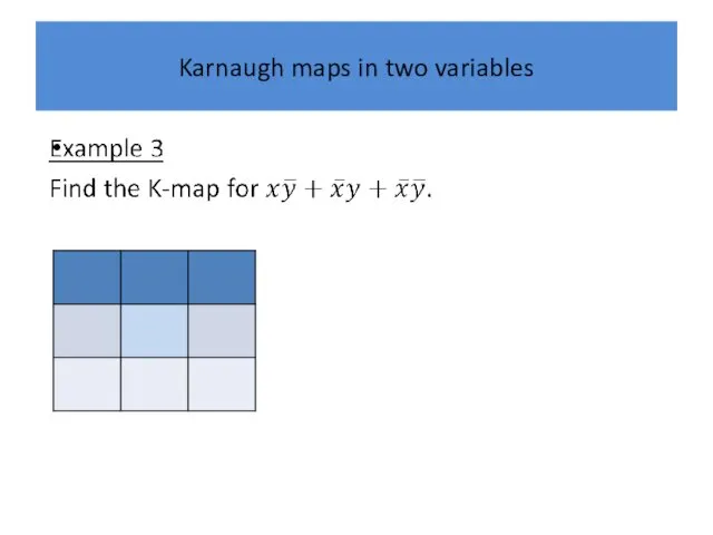
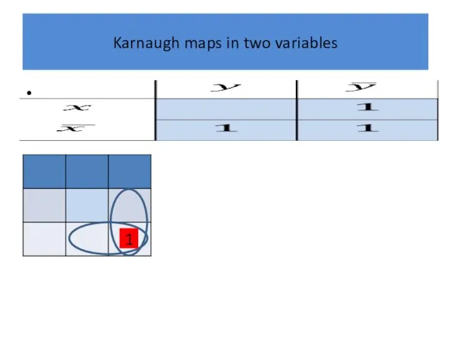
- 10. Karnaugh maps in two variables
- 11. Karnaugh maps in two variables
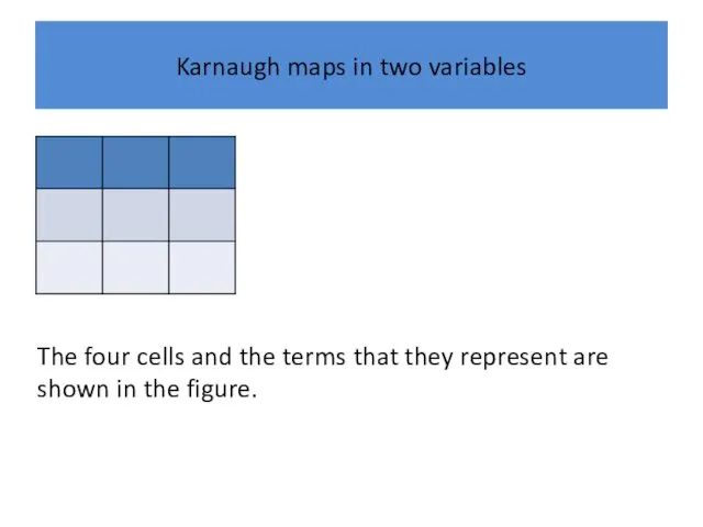
- 12. Karnaugh maps in two variables The four cells and the terms that they represent are shown
- 13. Karnaugh maps in two variables
- 14. Karnaugh maps in two variables
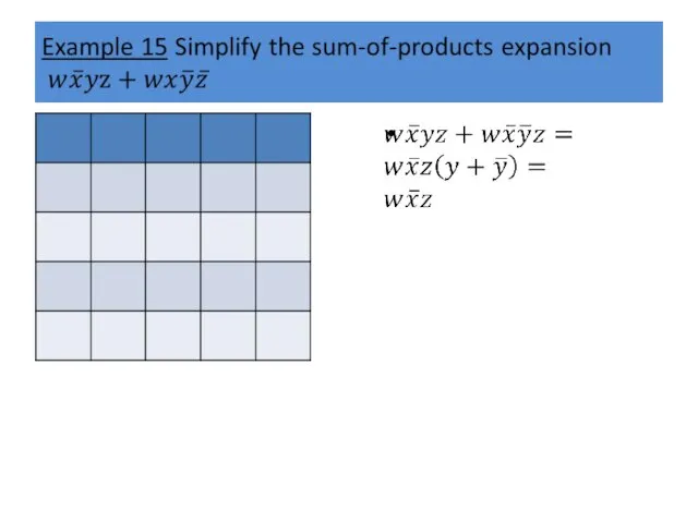
- 15. Karnaugh maps in two variables
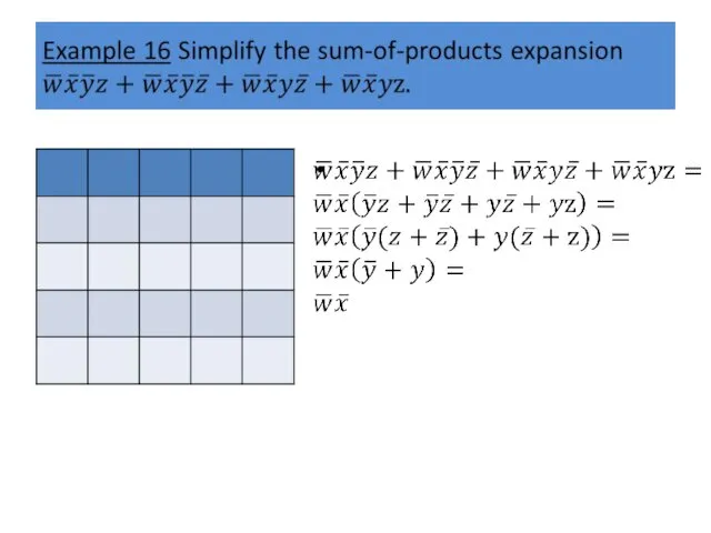
- 16. Karnaugh maps in two variables
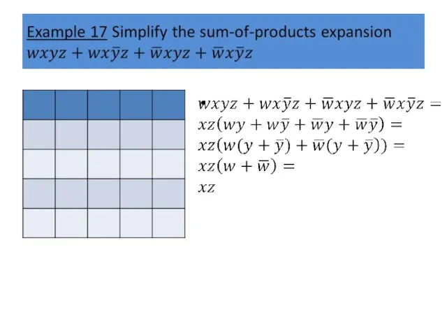
- 17. Karnaugh maps in two variables
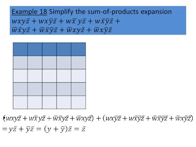
- 18. Karnaugh maps in two variables
- 19. Karnaugh maps in two variables
- 20. Karnaugh maps in two variables
- 21. Karnaugh maps in two variables 1
- 22. Karnaugh maps in two variables 1
- 23. Karnaugh maps in two variables 1
- 24. Karnaugh maps in two variables 1
- 25. Karnaugh maps in two variables 1
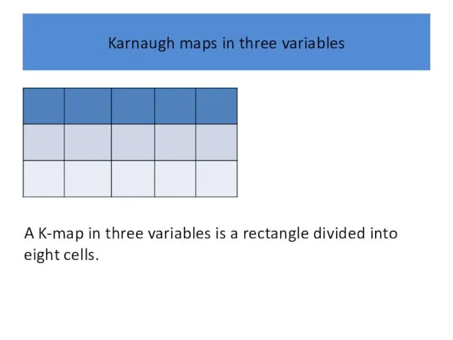
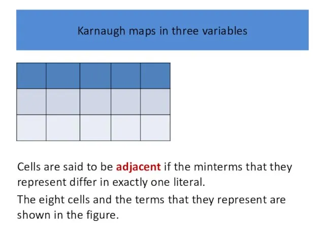
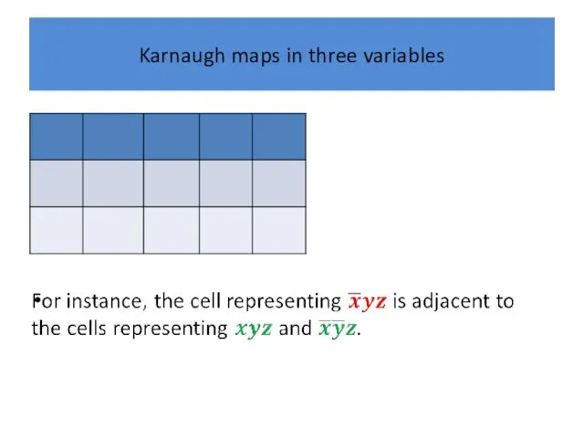
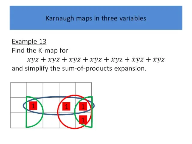
- 26. Karnaugh maps in three variables A K-map in three variables is a rectangle divided into eight
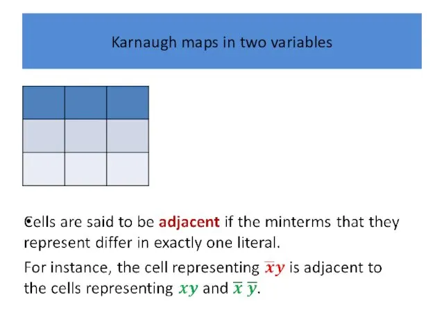
- 27. Karnaugh maps in three variables Cells are said to be adjacent if the minterms that they
- 28. Karnaugh maps in three variables
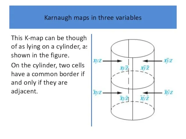
- 29. Karnaugh maps in three variables This K-map can be thought of as lying on a cylinder,
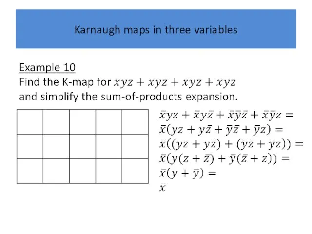
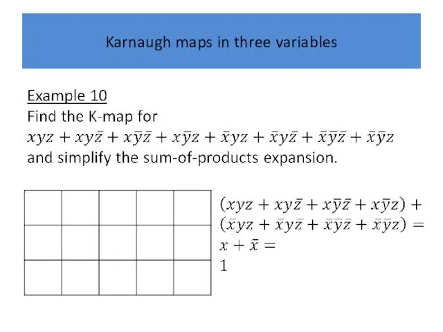
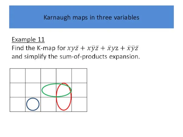
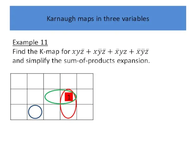
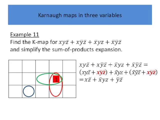
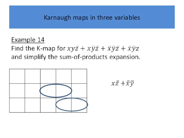
- 30. Karnaugh maps in three variables
- 31. Karnaugh maps in three variables
- 32. Karnaugh maps in three variables
- 33. Karnaugh maps in three variables
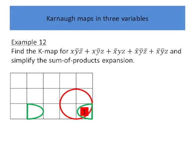
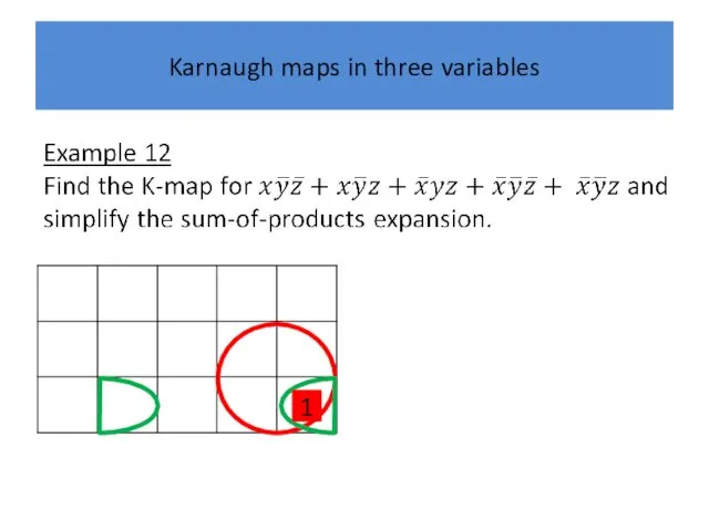
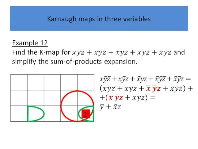
- 34. Karnaugh maps in three variables
- 35. Karnaugh maps in three variables
- 36. Karnaugh maps in three variables
- 37. Karnaugh maps in three variables
- 38. Karnaugh maps in three variables
- 39. Karnaugh maps in three variables 1
- 40. Karnaugh maps in three variables 1
- 41. Karnaugh maps in three variables 1
- 42. Karnaugh maps in three variables 1
- 43. Karnaugh maps in three variables 1
- 44. Karnaugh maps in three variables 1
- 45. Karnaugh maps in three variables 1
- 46. Karnaugh maps in three variables 1
- 47. Karnaugh maps in three variables 1 1 1 1
- 48. Karnaugh maps in three variables 1 1 1 1
- 49. Karnaugh maps in three variables 1 1 1 1
- 50. Karnaugh maps in three variables 1 1 1 1
- 51. Karnaugh maps in three variables
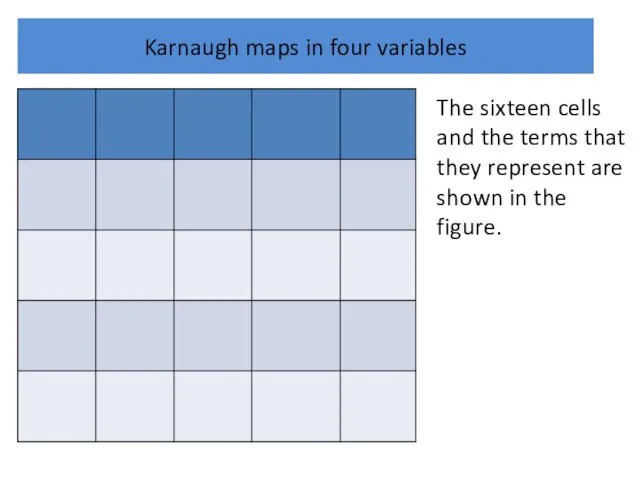
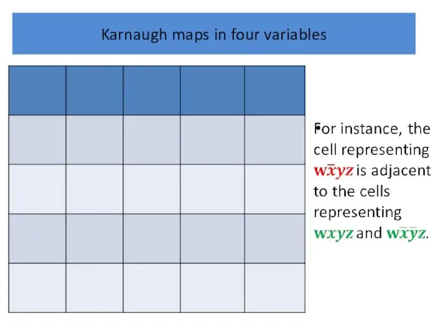
- 52. Karnaugh maps in four variables The sixteen cells and the terms that they represent are shown
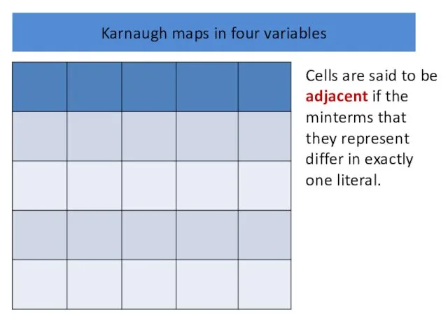
- 53. Karnaugh maps in four variables Cells are said to be adjacent if the minterms that they
- 54. Karnaugh maps in four variables
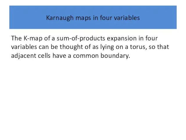
- 55. Karnaugh maps in four variables The K-map of a sum-of-products expansion in four variables can be
- 56. Karnaugh maps in four variables
- 57. Karnaugh maps in four variables
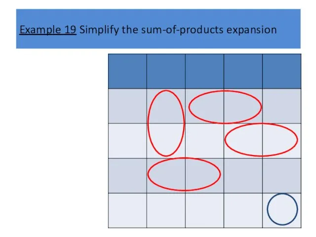
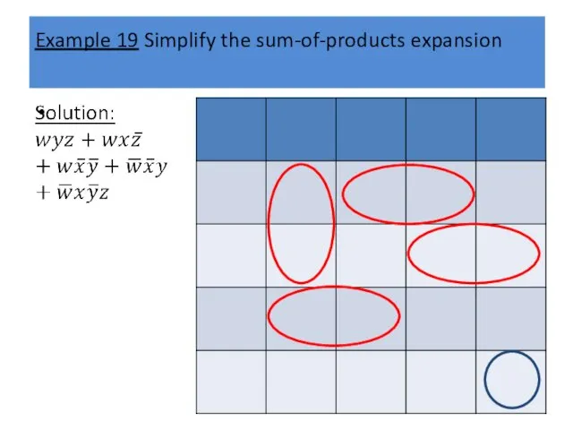
- 62. Example 19 Simplify the sum-of-products expansion
- 63. Example 19 Simplify the sum-of-products expansion
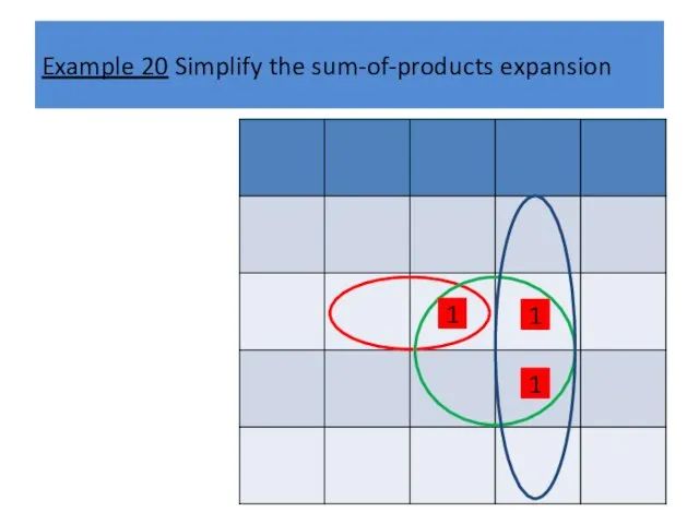
- 64. Example 20 Simplify the sum-of-products expansion 1 1 1
- 65. Example 20 Simplify the sum-of-products expansion 1 1 1
- 66. Example 20 Simplify the sum-of-products expansion 1 1 1
- 67. Example 20 Simplify the sum-of-products expansion 1 1 1
- 68. Example 20 Simplify the sum-of-products expansion 1 1 1
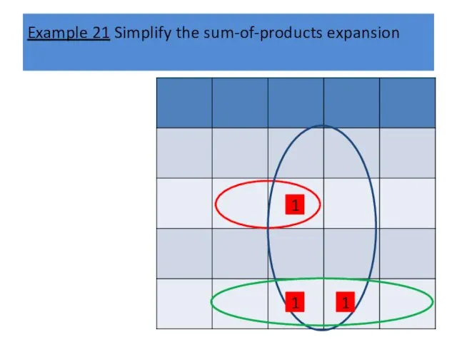
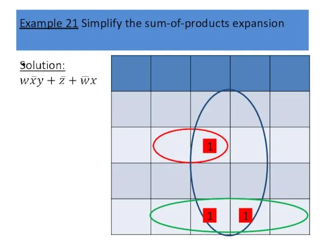
- 69. Example 21 Simplify the sum-of-products expansion 1 1 1
- 70. Example 21 Simplify the sum-of-products expansion 1 1 1
- 71. Example 21 Simplify the sum-of-products expansion 1 1 1
- 72. Example 21 Simplify the sum-of-products expansion 1 1 1
- 73. Example 21 Simplify the sum-of-products expansion 1 1 1
- 74. Circuits
- 75. Circuits The basic elements of circuits are called gates. Each type of gate implements a Boolean
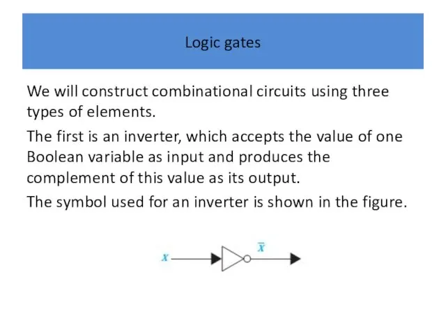
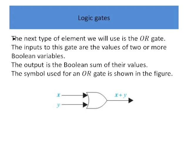
- 76. Logic gates We will construct combinational circuits using three types of elements. The first is an
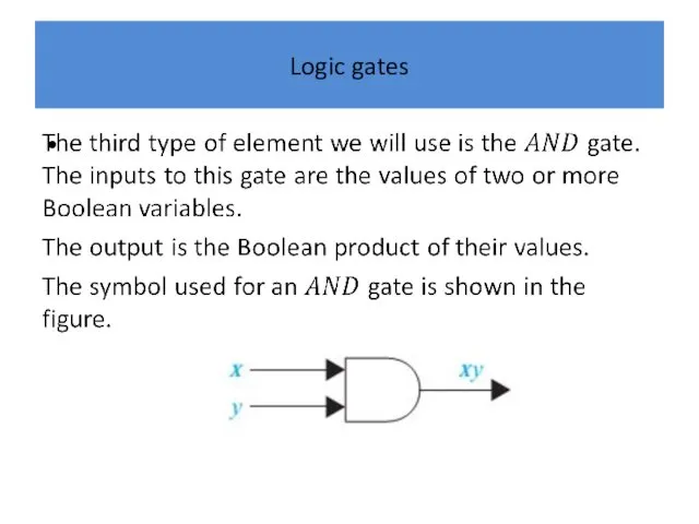
- 77. Logic gates
- 78. Logic gates
- 79. Circuits
- 80. Circuits The efficiency of a combinational circuit depends on the number and arrangement of its gates.
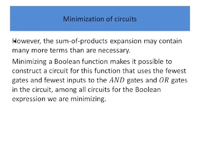
- 81. Minimization of circuits
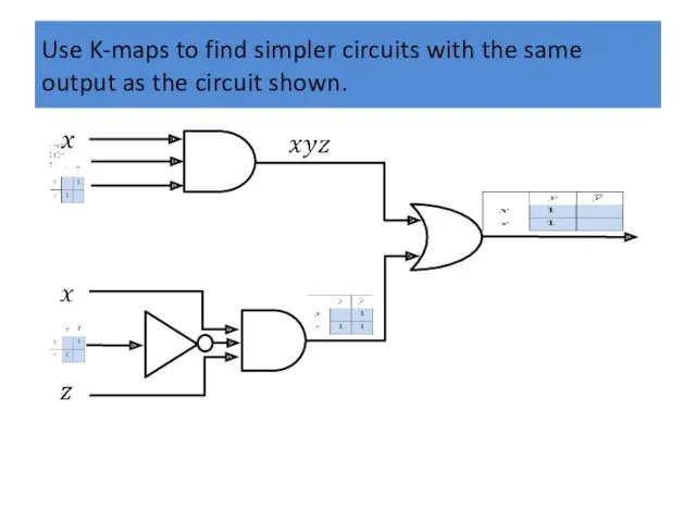
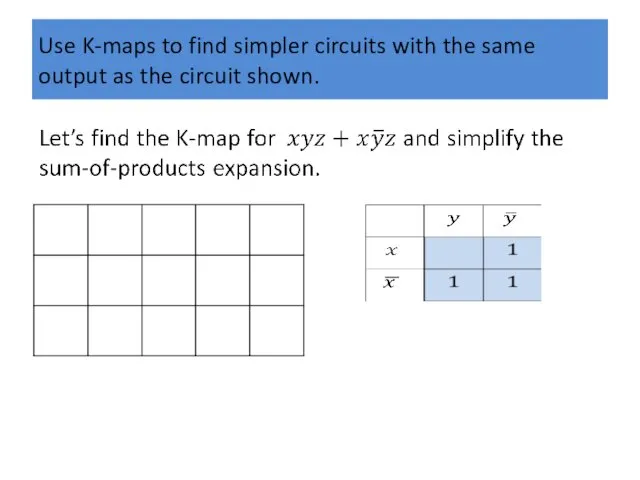
- 82. Use K-maps to find simpler circuits with the same output as the circuit shown.
- 83. Use K-maps to find simpler circuits with the same output as the circuit shown.
- 85. Скачать презентацию
Karnaugh maps
We will describe a procedure simplifying sum-of-products expansions.
The goal of
Karnaugh maps
We will describe a procedure simplifying sum-of-products expansions.
The goal of
Karnaugh maps
The procedure we will introduce, known as Karnaugh maps (or
Karnaugh maps
The procedure we will introduce, known as Karnaugh maps (or
Karnaugh maps
To reduce the number of terms in a Boolean expression
Karnaugh maps
To reduce the number of terms in a Boolean expression
Karnaugh maps
MAURICE KARNAUGH (BORN 1924)
Maurice Karnaugh, born in New York
Karnaugh maps
MAURICE KARNAUGH (BORN 1924)
Maurice Karnaugh, born in New York
Karnaugh maps
He was a member of the technical staff at Bell
Karnaugh maps
He was a member of the technical staff at Bell
Karnaugh maps
In 1970 he joined IBM as a member of the
Karnaugh maps
In 1970 he joined IBM as a member of the
Karnaugh maps
Karnaugh has made fundamental contributions to the application of digital
Karnaugh maps
Karnaugh has made fundamental contributions to the application of digital
Karnaugh maps
K-maps give us a visual method for simplifying sum-of-products expansions;
Karnaugh maps
K-maps give us a visual method for simplifying sum-of-products expansions;
Karnaugh maps in two variables
Karnaugh maps in two variables
Karnaugh maps in two variables
Karnaugh maps in two variables
Karnaugh maps in two variables
The four cells and the terms that
Karnaugh maps in two variables
The four cells and the terms that
Karnaugh maps in two variables
Karnaugh maps in two variables
Karnaugh maps in two variables
Karnaugh maps in two variables
Karnaugh maps in two variables
Karnaugh maps in two variables
Karnaugh maps in two variables
Karnaugh maps in two variables
Karnaugh maps in two variables
Karnaugh maps in two variables
Karnaugh maps in two variables
Karnaugh maps in two variables
Karnaugh maps in two variables
Karnaugh maps in two variables
Karnaugh maps in two variables
Karnaugh maps in two variables
Karnaugh maps in two variables
1
Karnaugh maps in two variables
1

Karnaugh maps in two variables
1
Karnaugh maps in two variables
1

Karnaugh maps in two variables
1
Karnaugh maps in two variables
1
Karnaugh maps in two variables
1
Karnaugh maps in two variables
1
Karnaugh maps in two variables
1
Karnaugh maps in two variables
1
Karnaugh maps in three variables
A K-map in three variables is a
Karnaugh maps in three variables
A K-map in three variables is a
Karnaugh maps in three variables
Cells are said to be adjacent if
Karnaugh maps in three variables
Cells are said to be adjacent if
Karnaugh maps in three variables
Karnaugh maps in three variables
Karnaugh maps in three variables
This K-map can be thought of as
Karnaugh maps in three variables
This K-map can be thought of as
Karnaugh maps in three variables
Karnaugh maps in three variables
Karnaugh maps in three variables
Karnaugh maps in three variables
Karnaugh maps in three variables
Karnaugh maps in three variables
Karnaugh maps in three variables
Karnaugh maps in three variables
Karnaugh maps in three variables
Karnaugh maps in three variables
Karnaugh maps in three variables
Karnaugh maps in three variables
Karnaugh maps in three variables
Karnaugh maps in three variables
Karnaugh maps in three variables
Karnaugh maps in three variables
Karnaugh maps in three variables
Karnaugh maps in three variables

Karnaugh maps in three variables
1
Karnaugh maps in three variables
1
Karnaugh maps in three variables
1
Karnaugh maps in three variables
1

Karnaugh maps in three variables
1
Karnaugh maps in three variables
1
Karnaugh maps in three variables
1
Karnaugh maps in three variables
1
Karnaugh maps in three variables
1
Karnaugh maps in three variables
1

Karnaugh maps in three variables
1
Karnaugh maps in three variables
1
Karnaugh maps in three variables
1
Karnaugh maps in three variables
1
Karnaugh maps in three variables
1
Karnaugh maps in three variables
1

Karnaugh maps in three variables
1
1
1
1
Karnaugh maps in three variables
1
1
1
1

Karnaugh maps in three variables
1
1
1
1
Karnaugh maps in three variables
1
1
1
1
Karnaugh maps in three variables
1
1
1
1
Karnaugh maps in three variables
1
1
1
1

Karnaugh maps in three variables
1
1
1
1
Karnaugh maps in three variables
1
1
1
1
Karnaugh maps in three variables
Karnaugh maps in three variables
Karnaugh maps in four variables
The sixteen cells and the terms that
Karnaugh maps in four variables
The sixteen cells and the terms that
Karnaugh maps in four variables
Cells are said to be adjacent if
Karnaugh maps in four variables
Cells are said to be adjacent if
Karnaugh maps in four variables
Karnaugh maps in four variables
Karnaugh maps in four variables
The K-map of a sum-of-products expansion in
Karnaugh maps in four variables
The K-map of a sum-of-products expansion in
Karnaugh maps in four variables
Karnaugh maps in four variables
Karnaugh maps in four variables
Karnaugh maps in four variables
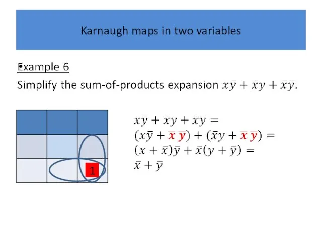
Example 19 Simplify the sum-of-products expansion
Example 19 Simplify the sum-of-products expansion
Example 19 Simplify the sum-of-products expansion
Example 19 Simplify the sum-of-products expansion

Example 20 Simplify the sum-of-products expansion
1
1
1
Example 20 Simplify the sum-of-products expansion
1
1
1
Example 20 Simplify the sum-of-products expansion
1
1
1
Example 20 Simplify the sum-of-products expansion
1
1
1

Example 20 Simplify the sum-of-products expansion
1
1
1
Example 20 Simplify the sum-of-products expansion
1
1
1

Example 20 Simplify the sum-of-products expansion
1
1
1
Example 20 Simplify the sum-of-products expansion
1
1
1

Example 20 Simplify the sum-of-products expansion
1
1
1
Example 20 Simplify the sum-of-products expansion
1
1
1
Example 21 Simplify the sum-of-products expansion
1
1
1
Example 21 Simplify the sum-of-products expansion
1
1
1

Example 21 Simplify the sum-of-products expansion
1
1
1
Example 21 Simplify the sum-of-products expansion
1
1
1

Example 21 Simplify the sum-of-products expansion
1
1
1
Example 21 Simplify the sum-of-products expansion
1
1
1

Example 21 Simplify the sum-of-products expansion
1
1
1
Example 21 Simplify the sum-of-products expansion
1
1
1
Example 21 Simplify the sum-of-products expansion
1
1
1
Example 21 Simplify the sum-of-products expansion
1
1
1
Circuits
Circuits
Circuits
The basic elements of circuits are called gates.
Each type of
Circuits
The basic elements of circuits are called gates.
Each type of
Logic gates
We will construct combinational circuits using three types of elements.
Logic gates
We will construct combinational circuits using three types of elements.
Logic gates
Logic gates
Logic gates
Logic gates
Circuits
Circuits
Circuits
The efficiency of a combinational circuit depends on the number and
Circuits
The efficiency of a combinational circuit depends on the number and
Minimization of circuits
Minimization of circuits
Use K-maps to find simpler circuits with the same output as
Use K-maps to find simpler circuits with the same output as
Use K-maps to find simpler circuits with the same output as
Use K-maps to find simpler circuits with the same output as
 Творческое задание интернет-проекта Путешествие в мир химии
 Предмет, функции и объект исследования социологии
 Система понятий дисциплины Литературное образование дошкольников
 Построение циклограммы. Основы поточной организации работ
 Разработка родительского собрания Наши дети не для насилия
 Учет кассовых операций
 Процесс пищеварения в ротовой полости
 Родительское собрание в подготовительной группе
 Проект Уберечь от дурмана
 Перша медична допомога
 Игры на развитие мышления
 Конвейер проектов – муниципальный конкурс проектов
 Спутниковые системы навигации. Угломерные бортовые РНС. Дальномерные РНС и радиовысотомеры
 Строение прокариотичекой клетки Айниятуллин Р.прБ-119
 Поздравление мамам
 презентация к мероприятию 9 мая
 Обогащение полезных ископаемых. Лекция 1-2
 Презентация День Победы.
 Republica de Cuba Cienfuegos y Santiago de Cuba
 Технологическая карта к занятию по теме Первые шаги в космос (Изготовление плоскостной ракеты со щелевидным соединением).
 Ұлттық діндер
 Строение и работа сердца
 презентация по внеурочной деятельности
 Метод проблемного обучения
 Исследовательская работа ученика 1 Б класса Хлапонина Захара Откуда у пчёл мёд?
 Электрохимические технологии неорганических веществ
 Определение соотношения составных частей и массы нетто консервов
 Белки, жиры и углеводы