- Types of algorithms

Содержание
- 2. Algorithm classification Algorithms that use a similar problem-solving approach can be grouped together This classification scheme
- 3. A short list of categories Algorithm types we will consider include: Simple recursive algorithms Backtracking algorithms
- 4. Simple recursive algorithms I A simple recursive algorithm: Solves the base cases directly Recurs with a
- 5. Example recursive algorithms To count the number of elements in a list: If the list is
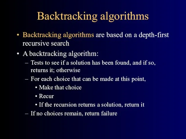
- 6. Backtracking algorithms Backtracking algorithms are based on a depth-first recursive search A backtracking algorithm: Tests to
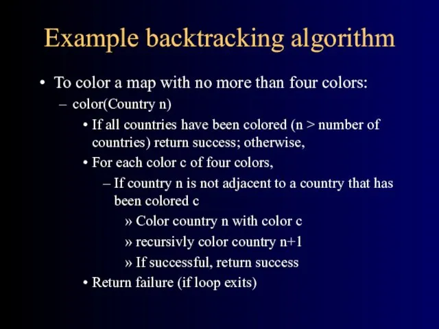
- 7. Example backtracking algorithm To color a map with no more than four colors: color(Country n) If
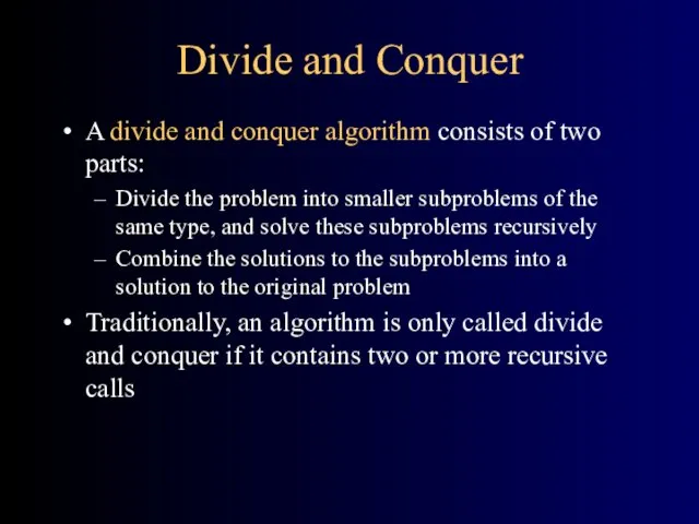
- 8. Divide and Conquer A divide and conquer algorithm consists of two parts: Divide the problem into
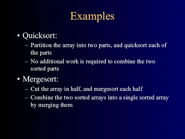
- 9. Examples Quicksort: Partition the array into two parts, and quicksort each of the parts No additional
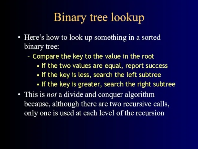
- 10. Binary tree lookup Here’s how to look up something in a sorted binary tree: Compare the
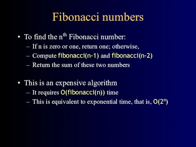
- 11. Fibonacci numbers To find the nth Fibonacci number: If n is zero or one, return one;
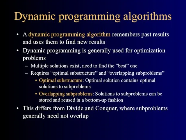
- 12. Dynamic programming algorithms A dynamic programming algorithm remembers past results and uses them to find new
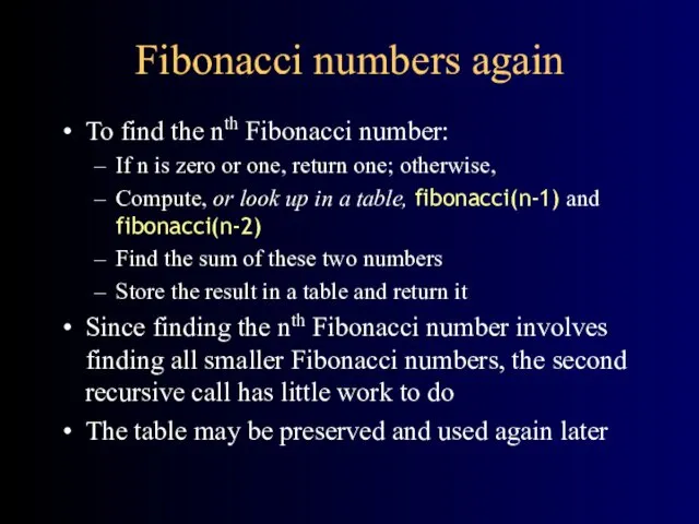
- 13. Fibonacci numbers again To find the nth Fibonacci number: If n is zero or one, return
- 14. Greedy algorithms An optimization problem is one in which you want to find, not just a
- 15. Example: Counting money Suppose you want to count out a certain amount of money, using the
- 16. A failure of the greedy algorithm In some (fictional) monetary system, “krons” come in 1 kron,
- 17. Branch and bound algorithms Branch and bound algorithms are generally used for optimization problems As the
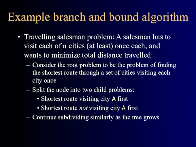
- 18. Example branch and bound algorithm Travelling salesman problem: A salesman has to visit each of n
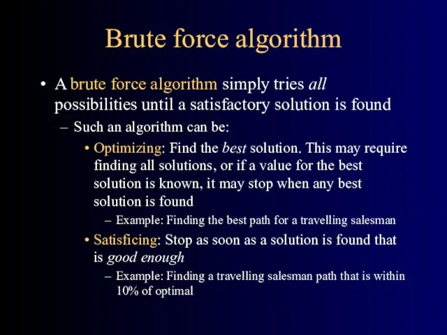
- 19. Brute force algorithm A brute force algorithm simply tries all possibilities until a satisfactory solution is
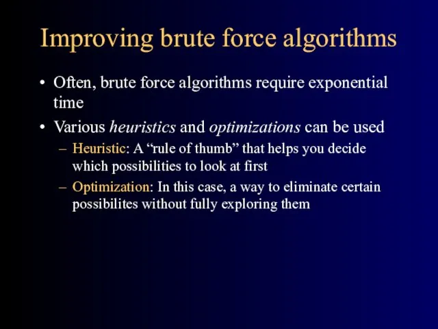
- 20. Improving brute force algorithms Often, brute force algorithms require exponential time Various heuristics and optimizations can
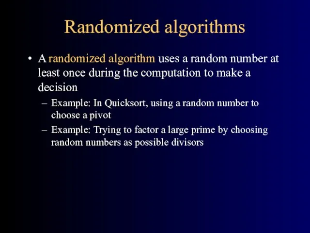
- 21. Randomized algorithms A randomized algorithm uses a random number at least once during the computation to
- 23. Скачать презентацию
Algorithm classification
Algorithms that use a similar problem-solving approach can be grouped
Algorithm classification
Algorithms that use a similar problem-solving approach can be grouped
A short list of categories
Algorithm types we will consider include:
Simple recursive
A short list of categories
Algorithm types we will consider include:
Simple recursive
Simple recursive algorithms I
A simple recursive algorithm:
Solves the base cases directly
Recurs
Simple recursive algorithms I
A simple recursive algorithm:
Solves the base cases directly
Recurs
Example recursive algorithms
To count the number of elements in a list:
If
Example recursive algorithms
To count the number of elements in a list:
If
Backtracking algorithms
Backtracking algorithms are based on a depth-first recursive search
A backtracking
Backtracking algorithms
Backtracking algorithms are based on a depth-first recursive search
A backtracking
Example backtracking algorithm
To color a map with no more than four
Example backtracking algorithm
To color a map with no more than four
Divide and Conquer
A divide and conquer algorithm consists of two parts:
Divide
Divide and Conquer
A divide and conquer algorithm consists of two parts:
Divide
Examples
Quicksort:
Partition the array into two parts, and quicksort each of the
Examples
Quicksort:
Partition the array into two parts, and quicksort each of the
Binary tree lookup
Here’s how to look up something in a sorted
Binary tree lookup
Here’s how to look up something in a sorted
Fibonacci numbers
To find the nth Fibonacci number:
If n is zero or
Fibonacci numbers
To find the nth Fibonacci number:
If n is zero or
Dynamic programming algorithms
A dynamic programming algorithm remembers past results and uses
Dynamic programming algorithms
A dynamic programming algorithm remembers past results and uses
Fibonacci numbers again
To find the nth Fibonacci number:
If n is zero
Fibonacci numbers again
To find the nth Fibonacci number:
If n is zero
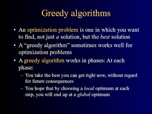
Greedy algorithms
An optimization problem is one in which you want to
Greedy algorithms
An optimization problem is one in which you want to
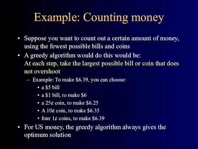
Example: Counting money
Suppose you want to count out a certain amount
Example: Counting money
Suppose you want to count out a certain amount
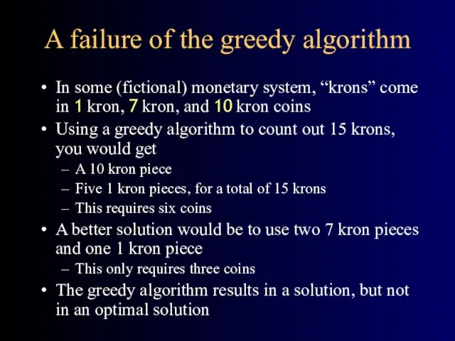
A failure of the greedy algorithm
In some (fictional) monetary system, “krons”
A failure of the greedy algorithm
In some (fictional) monetary system, “krons”
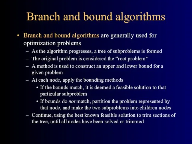
Branch and bound algorithms
Branch and bound algorithms are generally used for
Branch and bound algorithms
Branch and bound algorithms are generally used for
Example branch and bound algorithm
Travelling salesman problem: A salesman has to
Example branch and bound algorithm
Travelling salesman problem: A salesman has to
Brute force algorithm
A brute force algorithm simply tries all possibilities until
Brute force algorithm
A brute force algorithm simply tries all possibilities until
Improving brute force algorithms
Often, brute force algorithms require exponential time
Various heuristics
Improving brute force algorithms
Often, brute force algorithms require exponential time
Various heuristics
Randomized algorithms
A randomized algorithm uses a random number at least once
Randomized algorithms
A randomized algorithm uses a random number at least once
 Индивидуальная консультация для родителей. Воспитание самостоятельности у детей младшего дошкольного возраста
 Будущее (wecompress.com)
 Лаборатория социального проектирования
 Русские художественные промыслы
 Бусоград или волшебные игры Феи Бусинки
 Банкротство коммерческой организации и его прогнозирование
 Осложнения острого аппендицита. Гнойники брюшной полости
 Презентация к уроку 10 класса (базового) по химии 10 класс ТемаКаменный уголь. Фенол
 Рак шейки матки
 20190527_atstekskiy_kalendar
 Скребковые перегружатели
 429e21918e4fb5b5796faa520e64e332
 Коробочные страховые продукты. Рабочая тетрадь Банк ВТБ
 День борьбы со СПИДом
 Энергия топлива. Удельная теплота сгорания
 Мастер – класс по изготовлению дидактической игрушки для
 Чудотворцы
 Алгоритм. Свойства алгоритма. Способы описания алгоритмов
 Медицинское страхование. Медицинское страхование в системе социального страхования
 Презентация Весенние именинники
 трофимчук
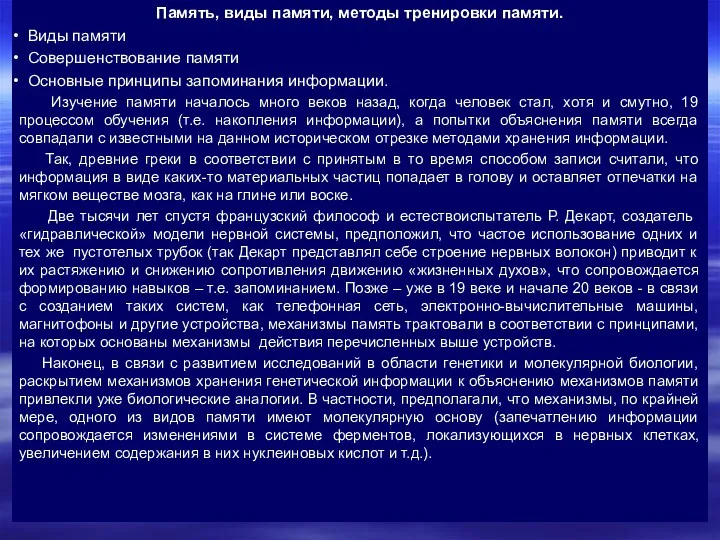 Память, виды и методы тренировки памяти
 Моя Педагогическая династия
 Презентация ко Дню Матери
 Криминалистическое почерковедение и автороведение
 Транспортная инфраструктура
 Закаливание. Методы закаливания
 Тест по математике за первое полугодие для 1 класса