- Capital Market History and Risk & Return

Содержание
- 2. A2. Capital Market History and Risk & Return (continued) Expected Returns and Variances Portfolios Announcements, Surprises,
- 3. A3. Risk, Return, and Financial Markets “. . . Wall Street shapes Main Street. Financial markets
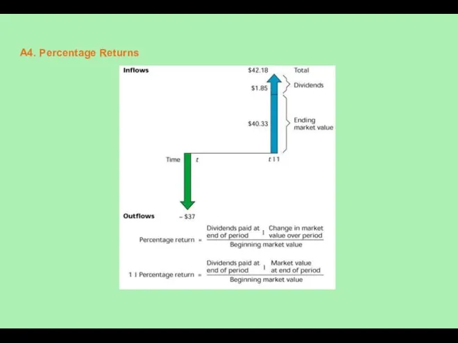
- 4. A4. Percentage Returns
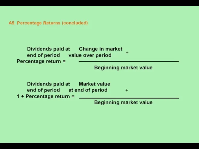
- 5. A5. Percentage Returns (concluded) Dividends paid at Change in market end of period value over period
- 6. A6. A $1 Investment in Different Types of Portfolios: 1926-1998
- 7. A7. Year-to-Year Total Returns on Large Company Common Stocks: 1926-1998
- 8. A8. Year-to-Year Total Returns on Small Company Common Stocks: 1926-1998
- 9. A9. Year-to-Year Total Returns on Bonds and Bills: 1926-1998
- 10. A10. Year-to-Year Total Returns on Bonds and Bills: 1926-1998 (concluded) Total Returns (%) 16 14 12
- 11. A11. Year-to-Year Inflation: 1926-1998
- 12. A12. Historical Dividend Yield on Common Stocks 10% 9 8 7 6 5 4 3 2
- 13. A13. S&P 500 Risk Premiums: 1926-1998
- 14. A14. Small Stock Risk Premiums: 1926-1998
- 15. A15. Using Capital Market History Now let’s use our knowledge of capital market history to make
- 16. A16. Using Capital Market History (continued) Risk premiums: First, we calculate risk premiums. The risk premium
- 17. A17. Using Capital Market History (continued) Risk premiums: First, we calculate risk premiums. The risk premium
- 18. A18. Using Capital Market History (concluded) Let’s return to our earlier questions. Suppose the current T-bill
- 19. A19. Average Annual Returns and Risk Premiums: 1926-1998 Investment Average Return Risk Premium Large-company stocks 13.2%
- 20. A20. Frequency Distribution of Returns on Common Stocks, 1926-1998
- 21. A21. Historical Returns, Standard Deviations, and Frequency Distributions: 1926-1998
- 22. A22. The Normal Distribution
- 23. A23. Two Views on Market Efficiency “ . . . in price movements . . .
- 24. A24. Stock Price Reaction to New Information in Efficient and Inefficient Markets Efficient market reaction: The
- 25. A25. A Quick Quiz Here are three questions that should be easy to answer (if you’ve
- 26. A26. Chapter 12 Quick Quiz (continued) 1. How are average annual returns measured? Annual returns are
- 27. A27. Chapter 12 Quick Quiz (continued) 2. How is volatility measured? Given a normal distribution, volatility
- 28. A28. Chapter 12 Quick Quiz (concluded) 3. Assume your portfolio has had returns of 11%, -8%,
- 29. A29. A Few Examples Suppose a stock had an initial price of $58 per share, paid
- 30. A30. A Few Examples (continued) Suppose a stock had an initial price of $58 per share,
- 31. A31. A Few Examples (continued) Using the following returns, calculate the average returns, the variances, and
- 32. A32. A Few Examples (continued) Mean return on X = (.18 + .11 - .09 +
- 33. A33. A Few Examples (concluded) Mean return on X = (.18 + .11 - .09 +
- 34. A34. Expected Return and Variance: Basic Ideas The quantification of risk and return is a crucial
- 35. A35. Example: Calculating the Expected Return pi Ri Probability Return in State of Economy of state
- 36. A36. Example: Calculating the Expected Return (concluded) i (pi × Ri) i = 1 -1.25% i
- 37. A37. Calculation of Expected Return Stock L Stock U (3) (5) (2) Rate of Rate of
- 38. A38. Example: Calculating the Variance pi ri Probability Return in State of Economy of state i
- 39. A39. Calculating the Variance (concluded) i (Ri - R)2 pi × (Ri - R)2 i=1 .04
- 40. A40. Example: Expected Returns and Variances State of the Probability Return on Return on economy of
- 41. A41. Example: Expected Returns and Variances (concluded) B. Variances Var(RA) = 0.40 × (.30 - .06)2
- 42. A42. Example: Portfolio Expected Returns and Variances Portfolio weights: put 50% in Asset A and 50%
- 43. A43. Example: Portfolio Expected Returns and Variances (continued) A. E(RP) = 0.40 × (.125) + 0.60
- 44. A44. Example: Portfolio Expected Returns and Variances (concluded) New portfolio weights: put 3/7 in A and
- 45. A45. The Effect of Diversification on Portfolio Variance Stock A returns 0.05 0.04 0.03 0.02 0.01
- 46. A46. Announcements, Surprises, and Expected Returns Key issues: What are the components of the total return?
- 47. A47. Risk: Systematic and Unsystematic Systematic and Unsystematic Risk Types of surprises 1. Systematic or “market”
- 48. A48. Peter Bernstein on Risk and Diversification “Big risks are scary when you cannot diversify them,
- 49. A49. Standard Deviations of Annual Portfolio Returns ( 3) (2) Ratio of Portfolio (1) Average Standard
- 50. A50. Portfolio Diversification
- 51. A51. Beta Coefficients for Selected Companies Beta Company Coefficient American Electric Power .65 Exxon .80 IBM
- 52. A52. Example: Portfolio Beta Calculations Amount Portfolio Stock Invested Weights Beta (1) (2) (3) (4) (3)
- 53. A53. Example: Portfolio Expected Returns and Betas Assume you wish to hold a portfolio consisting of
- 54. A54. Example: Portfolio Expected Returns and Betas (concluded) Proportion Proportion Portfolio Invested in Invested in Expected
- 55. A55. Return, Risk, and Equilibrium Key issues: What is the relationship between risk and return? What
- 56. A56. Return, Risk, and Equilibrium (concluded) Example: Asset A has an expected return of 12% and
- 57. A57. Return, Risk, and Equilibrium (concluded) Example: Asset A has an expected return of 12% and
- 58. A58. The Capital Asset Pricing Model The Capital Asset Pricing Model (CAPM) - an equilibrium model
- 59. A59. The Security Market Line (SML)
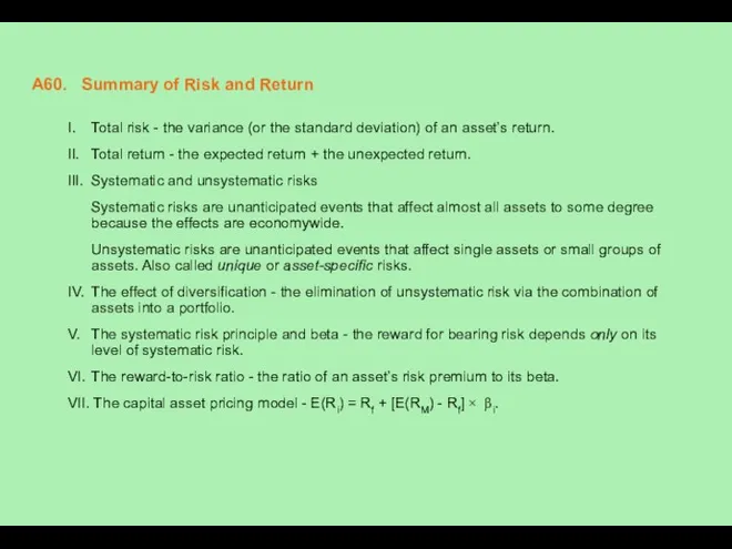
- 60. A60. Summary of Risk and Return I. Total risk - the variance (or the standard deviation)
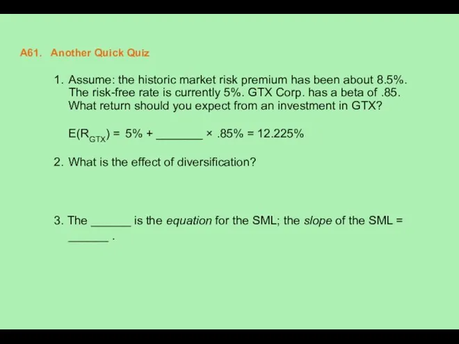
- 61. A61. Another Quick Quiz 1. Assume: the historic market risk premium has been about 8.5%. The
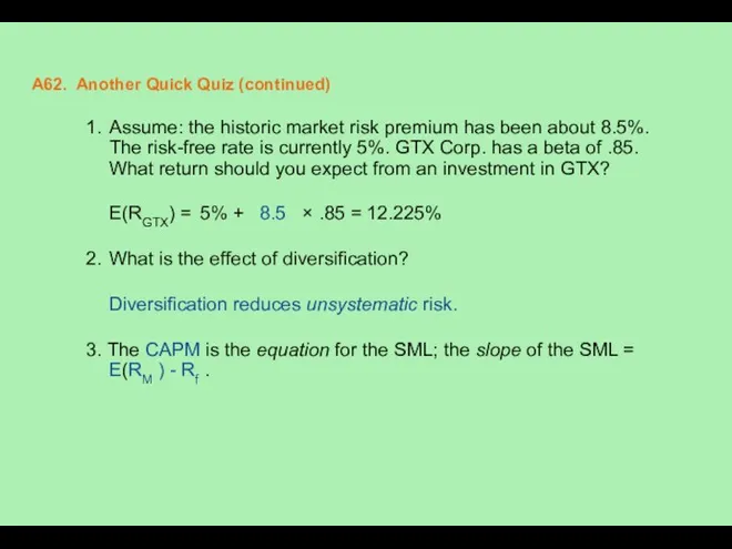
- 62. A62. Another Quick Quiz (continued) 1. Assume: the historic market risk premium has been about 8.5%.
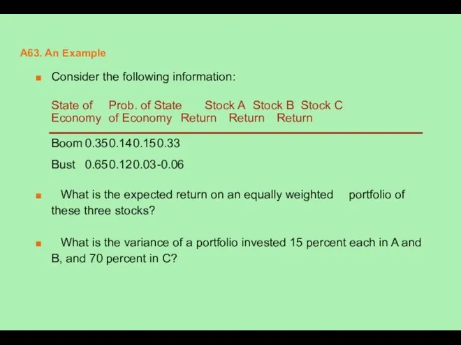
- 63. A63. An Example Consider the following information: State of Prob. of State Stock A Stock B
- 64. A64. Solution to the Example Expected returns on an equal-weighted portfolio a. Boom E[Rp] = (.14
- 65. A65. Solution to the Example (continued) b. Boom: E[Rp] = __ (.14) + .15(.15) + .70(.33)
- 66. A66. Solution to the Example (concluded) b. Boom: E[Rp] = .15(.14) + .15(.15) + .70(.33) =
- 67. A67. Another Example Using information from capital market history, determine the return on a portfolio that
- 69. Скачать презентацию
A2. Capital Market History and Risk & Return (continued)
Expected Returns
A2. Capital Market History and Risk & Return (continued)
Expected Returns
A3. Risk, Return, and Financial Markets
“. . . Wall Street
A3. Risk, Return, and Financial Markets
“. . . Wall Street
A4. Percentage Returns
A4. Percentage Returns
A5. Percentage Returns (concluded)
Dividends paid at Change in market
end of
A5. Percentage Returns (concluded)
Dividends paid at Change in market end of
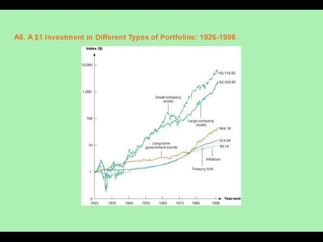
A6. A $1 Investment in Different Types of Portfolios: 1926-1998
A6. A $1 Investment in Different Types of Portfolios: 1926-1998
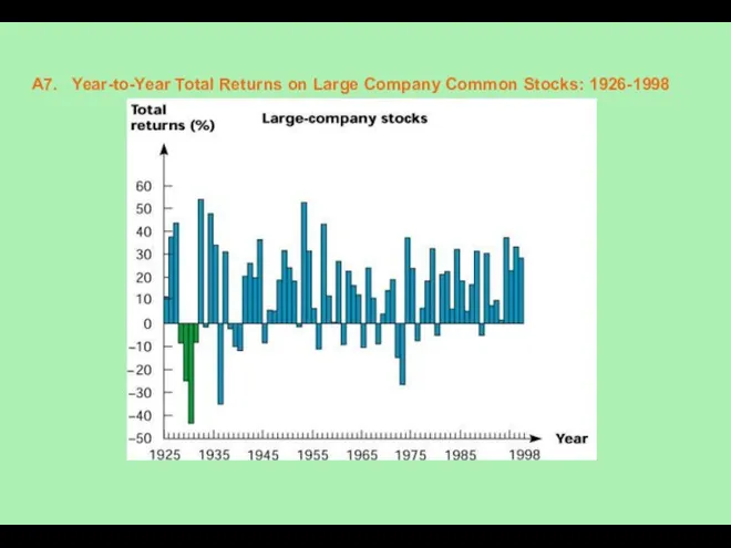
A7. Year-to-Year Total Returns on Large Company Common Stocks: 1926-1998
A7. Year-to-Year Total Returns on Large Company Common Stocks: 1926-1998
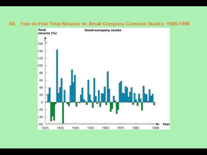
A8. Year-to-Year Total Returns on Small Company Common Stocks: 1926-1998
A8. Year-to-Year Total Returns on Small Company Common Stocks: 1926-1998
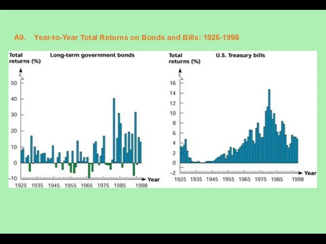
A9. Year-to-Year Total Returns on Bonds and Bills: 1926-1998
A9. Year-to-Year Total Returns on Bonds and Bills: 1926-1998
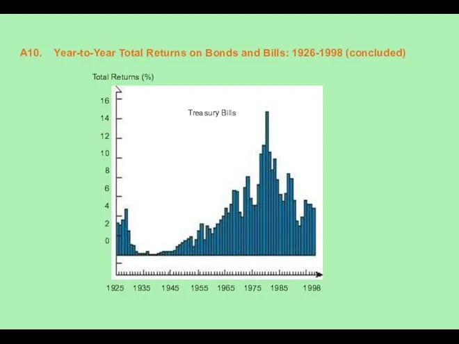
A10. Year-to-Year Total Returns on Bonds and Bills: 1926-1998 (concluded)
Total Returns
A10. Year-to-Year Total Returns on Bonds and Bills: 1926-1998 (concluded)
Total Returns
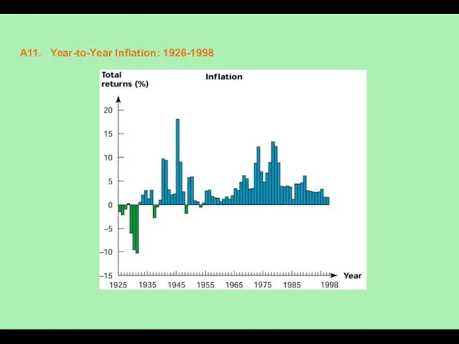
A11. Year-to-Year Inflation: 1926-1998
A11. Year-to-Year Inflation: 1926-1998
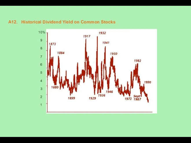
A12. Historical Dividend Yield on Common Stocks
10%
9
8
7
6
5
4
3
A12. Historical Dividend Yield on Common Stocks
10%
9
8
7
6
5
4
3
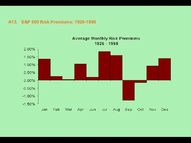
A13. S&P 500 Risk Premiums: 1926-1998
A13. S&P 500 Risk Premiums: 1926-1998
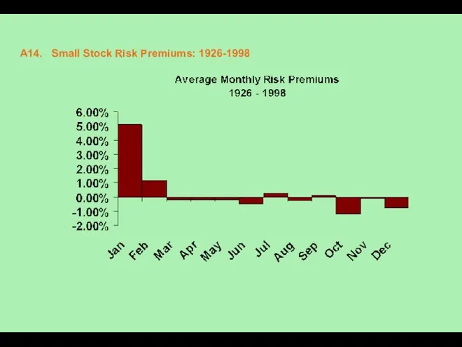
A14. Small Stock Risk Premiums: 1926-1998
A14. Small Stock Risk Premiums: 1926-1998
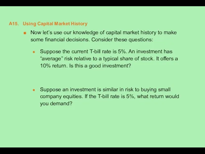
A15. Using Capital Market History
Now let’s use our knowledge of capital
A15. Using Capital Market History
Now let’s use our knowledge of capital
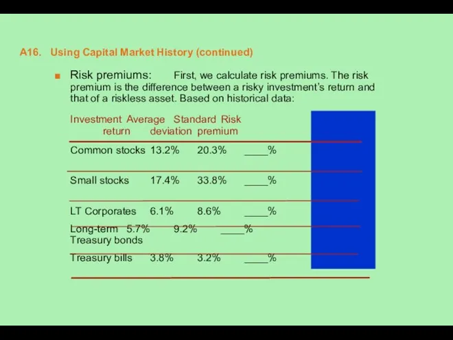
A16. Using Capital Market History (continued)
Risk premiums: First, we calculate risk
A16. Using Capital Market History (continued)
Risk premiums: First, we calculate risk
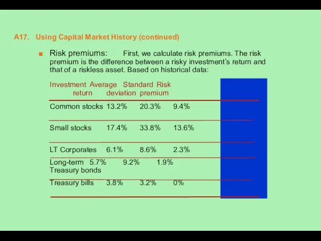
A17. Using Capital Market History (continued)
Risk premiums: First, we calculate risk
A17. Using Capital Market History (continued)
Risk premiums: First, we calculate risk
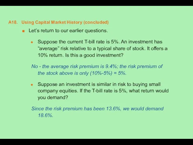
A18. Using Capital Market History (concluded)
Let’s return to our earlier questions.
Suppose
A18. Using Capital Market History (concluded)
Let’s return to our earlier questions.
Suppose
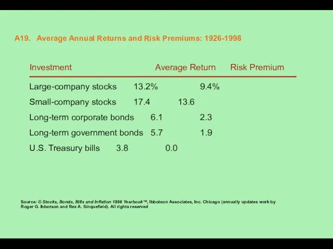
A19. Average Annual Returns and Risk Premiums: 1926-1998
Investment Average Return Risk
A19. Average Annual Returns and Risk Premiums: 1926-1998
Investment Average Return Risk
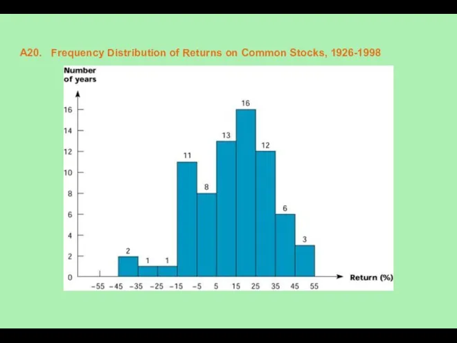
A20. Frequency Distribution of Returns on Common Stocks, 1926-1998
A20. Frequency Distribution of Returns on Common Stocks, 1926-1998
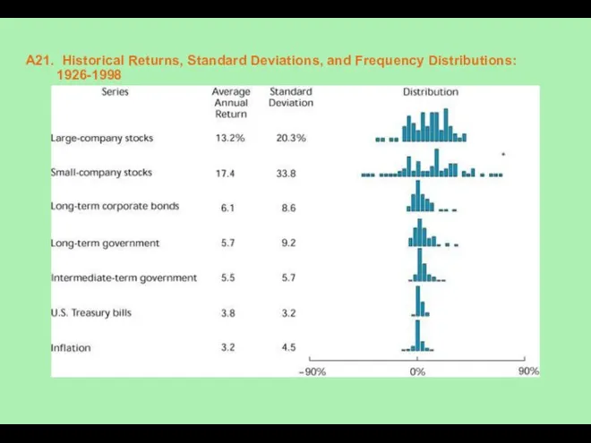
A21. Historical Returns, Standard Deviations, and Frequency Distributions:
1926-1998
A21. Historical Returns, Standard Deviations, and Frequency Distributions:
1926-1998

A22. The Normal Distribution
A22. The Normal Distribution
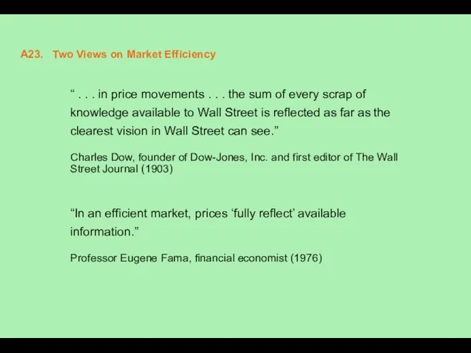
A23. Two Views on Market Efficiency
“ . . . in price
A23. Two Views on Market Efficiency
“ . . . in price
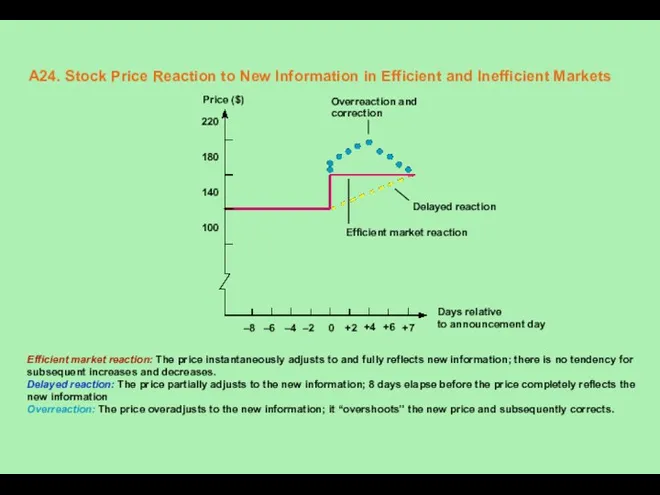
A24. Stock Price Reaction to New Information in Efficient and Inefficient
A24. Stock Price Reaction to New Information in Efficient and Inefficient
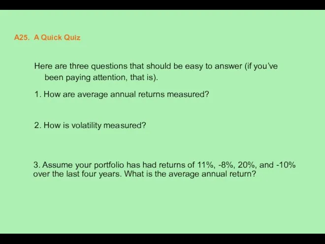
A25. A Quick Quiz
Here are three questions that should be easy
A25. A Quick Quiz
Here are three questions that should be easy
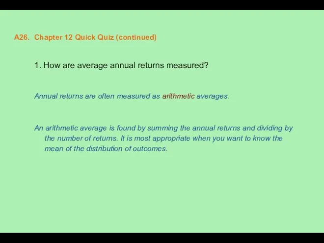
A26. Chapter 12 Quick Quiz (continued)
1. How are average annual returns
A26. Chapter 12 Quick Quiz (continued)
1. How are average annual returns
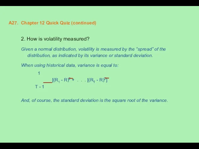
A27. Chapter 12 Quick Quiz (continued)
2. How is volatility measured?
Given a
A27. Chapter 12 Quick Quiz (continued)
2. How is volatility measured?
Given a
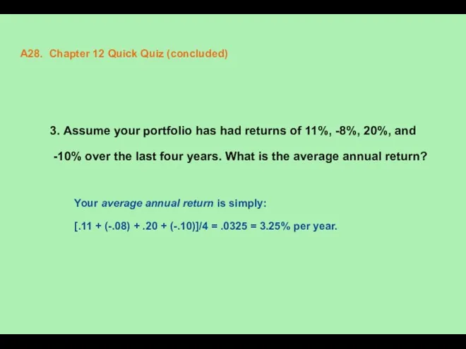
A28. Chapter 12 Quick Quiz (concluded)
3. Assume your portfolio has had
A28. Chapter 12 Quick Quiz (concluded)
3. Assume your portfolio has had
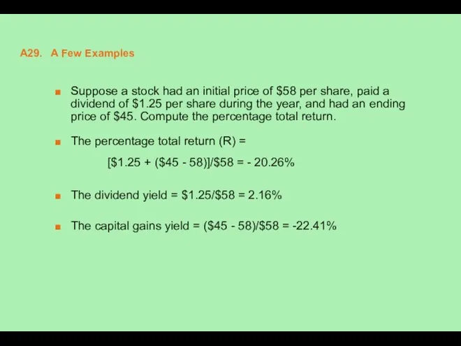
A29. A Few Examples
Suppose a stock had an initial price of
A29. A Few Examples
Suppose a stock had an initial price of
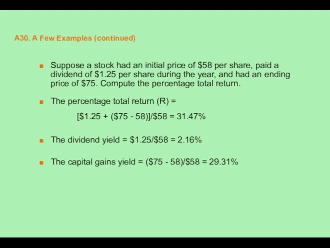
A30. A Few Examples (continued)
Suppose a stock had an initial price
A30. A Few Examples (continued)
Suppose a stock had an initial price
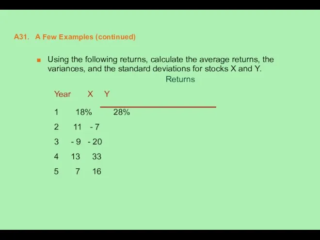
A31. A Few Examples (continued)
Using the following returns, calculate the average
A31. A Few Examples (continued)
Using the following returns, calculate the average
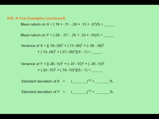
A32. A Few Examples (continued)
Mean return on X = (.18 +
A32. A Few Examples (continued)
Mean return on X = (.18 +
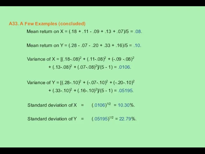
A33. A Few Examples (concluded)
Mean return on X = (.18 +
A33. A Few Examples (concluded)
Mean return on X = (.18 +
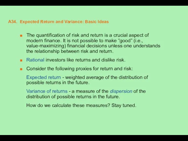
A34. Expected Return and Variance: Basic Ideas
The quantification of risk and
A34. Expected Return and Variance: Basic Ideas
The quantification of risk and
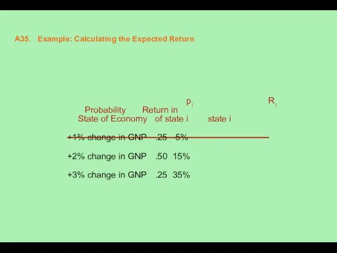
A35. Example: Calculating the Expected Return
pi Ri
Probability Return in
State of Economy of
A35. Example: Calculating the Expected Return
pi Ri
Probability Return in
State of Economy of
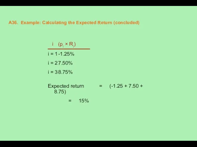
A36. Example: Calculating the Expected Return (concluded)
i (pi × Ri)
i =
A36. Example: Calculating the Expected Return (concluded)
i (pi × Ri)
i =
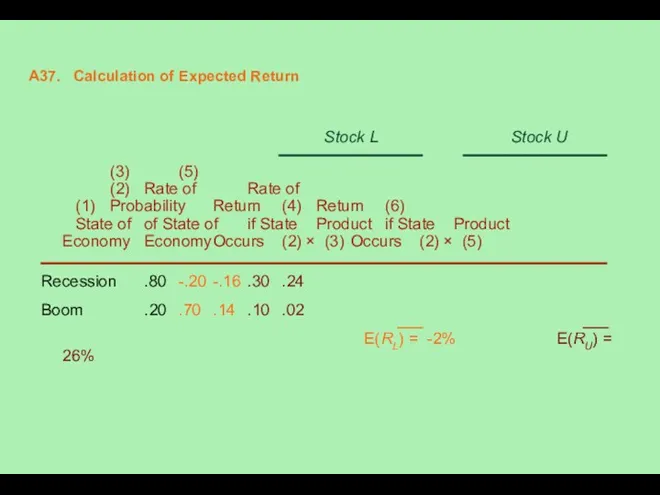
A37. Calculation of Expected Return
Stock L Stock U
(3) (5)
(2) Rate
A37. Calculation of Expected Return
Stock L Stock U
(3) (5)
(2) Rate
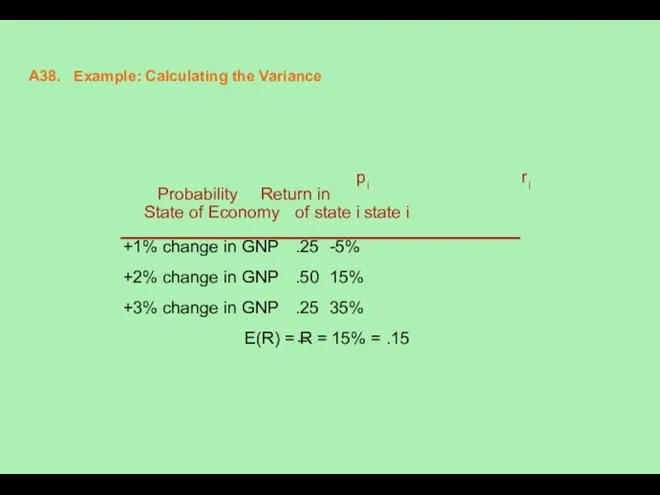
A38. Example: Calculating the Variance
pi ri
Probability Return in
State of Economy of
A38. Example: Calculating the Variance
pi ri
Probability Return in
State of Economy of
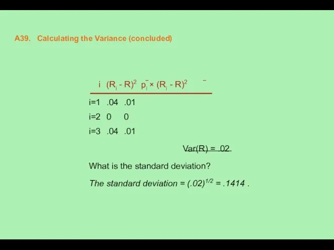
A39. Calculating the Variance (concluded)
i (Ri - R)2 pi × (Ri
A39. Calculating the Variance (concluded)
i (Ri - R)2 pi × (Ri
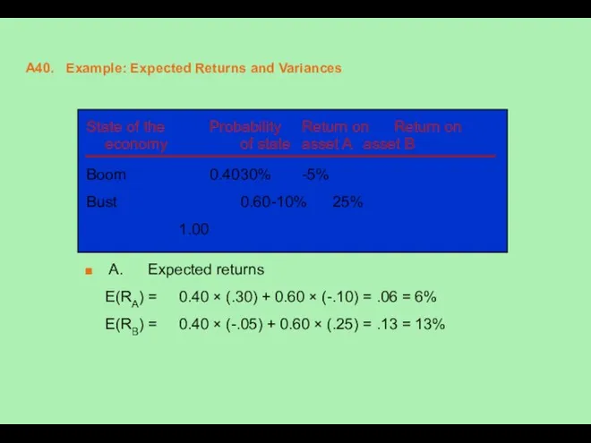
A40. Example: Expected Returns and Variances
State of the Probability Return on Return on
economy of state asset
A40. Example: Expected Returns and Variances
State of the Probability Return on Return on economy of state asset
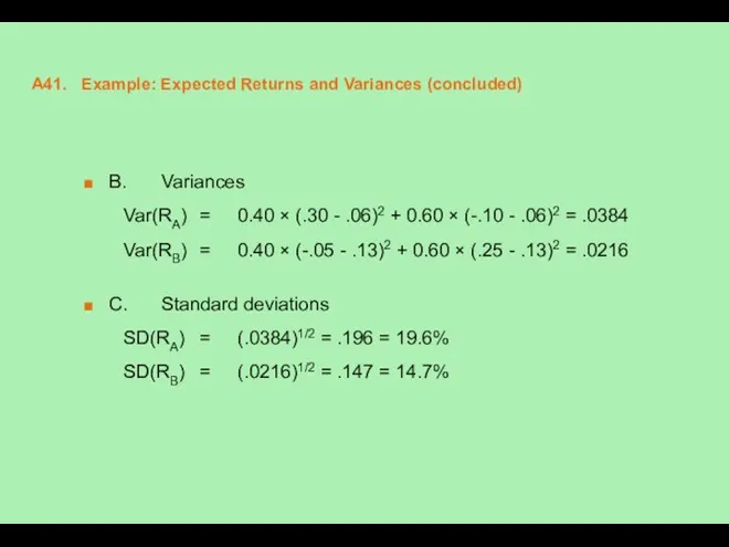
A41. Example: Expected Returns and Variances (concluded)
B. Variances
Var(RA) = 0.40 ×
A41. Example: Expected Returns and Variances (concluded)
B. Variances
Var(RA) = 0.40 ×
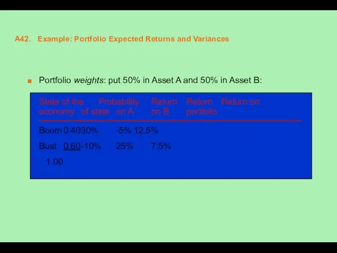
A42. Example: Portfolio Expected Returns and Variances
Portfolio weights: put 50% in
A42. Example: Portfolio Expected Returns and Variances
Portfolio weights: put 50% in
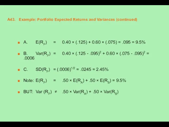
A43. Example: Portfolio Expected Returns and Variances (continued)
A. E(RP) = 0.40 ×
A43. Example: Portfolio Expected Returns and Variances (continued)
A. E(RP) = 0.40 ×
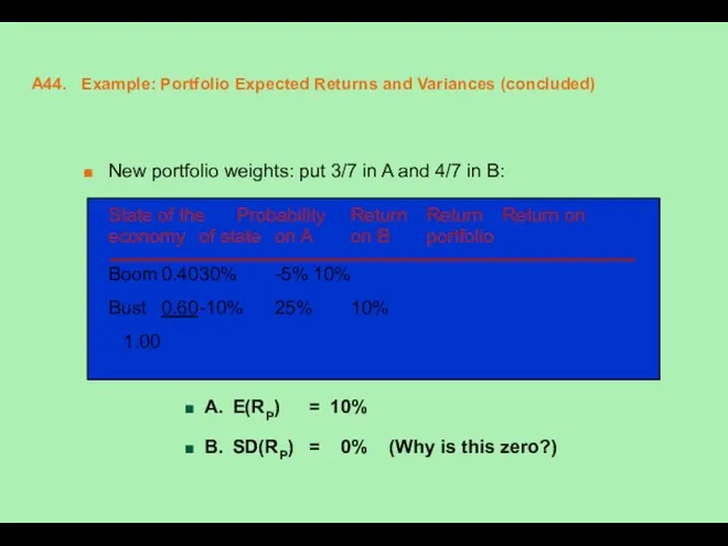
A44. Example: Portfolio Expected Returns and Variances (concluded)
New portfolio weights: put
A44. Example: Portfolio Expected Returns and Variances (concluded)
New portfolio weights: put
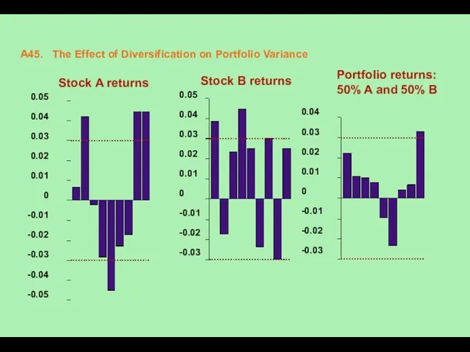
A45. The Effect of Diversification on Portfolio Variance
Stock A returns
0.05
0.04
0.03
0.02
0.01
0
-0.01
-0.02
-0.03
-0.04
-0.05
0.05
0.04
0.03
0.02
0.01
0
-0.01
-0.02
-0.03
Stock B
A45. The Effect of Diversification on Portfolio Variance
Stock A returns
0.05
0.04
0.03
0.02
0.01
0
-0.01
-0.02
-0.03
-0.04
-0.05
0.05
0.04
0.03
0.02
0.01
0
-0.01
-0.02
-0.03
Stock B
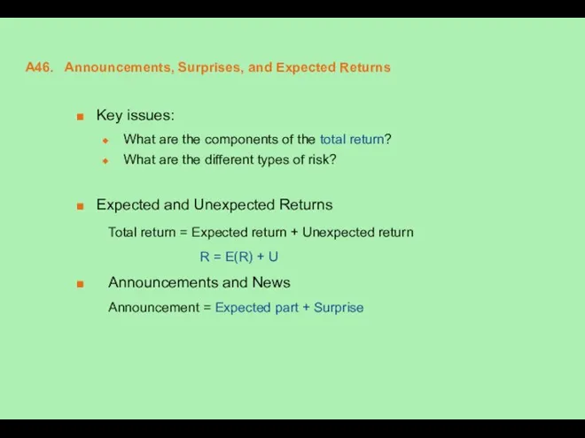
A46. Announcements, Surprises, and Expected Returns
Key issues:
What are the components of
A46. Announcements, Surprises, and Expected Returns
Key issues:
What are the components of
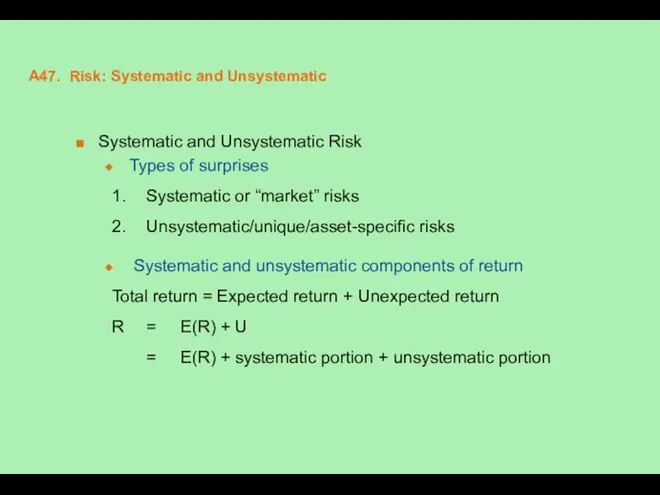
A47. Risk: Systematic and Unsystematic
Systematic and Unsystematic Risk
Types of surprises
1. Systematic
A47. Risk: Systematic and Unsystematic
Systematic and Unsystematic Risk
Types of surprises
1. Systematic

A48. Peter Bernstein on Risk and Diversification
“Big risks are scary
A48. Peter Bernstein on Risk and Diversification
“Big risks are scary
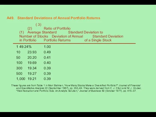
A49. Standard Deviations of Annual Portfolio Returns
( 3)
(2) Ratio of
A49. Standard Deviations of Annual Portfolio Returns
( 3) (2) Ratio of
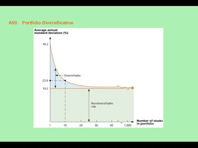
A50. Portfolio Diversification
A50. Portfolio Diversification
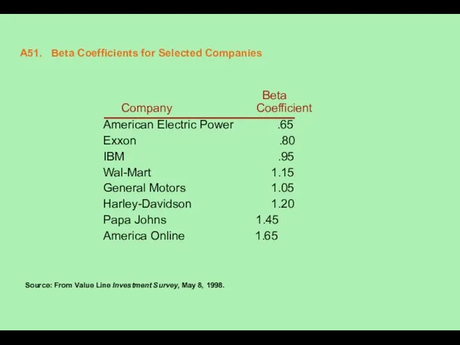
A51. Beta Coefficients for Selected Companies
Beta Company Coefficient
American Electric Power
A51. Beta Coefficients for Selected Companies
Beta Company Coefficient
American Electric Power
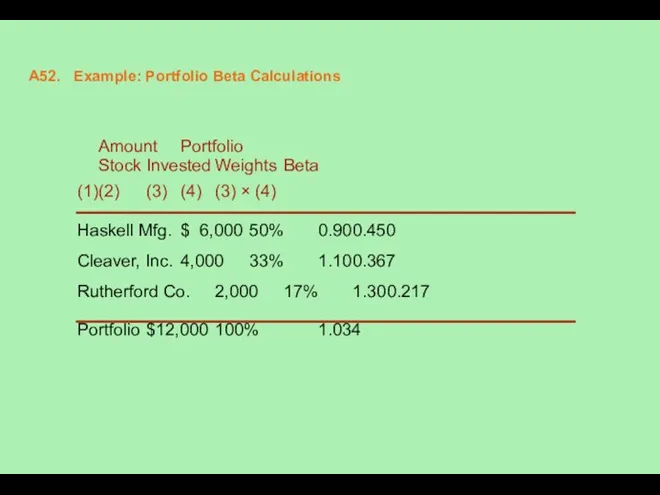
A52. Example: Portfolio Beta Calculations
Amount Portfolio
Stock Invested Weights Beta
(1) (2) (3) (4) (3) × (4)
Haskell Mfg. $ 6,000 50% 0.90 0.450
Cleaver,
A52. Example: Portfolio Beta Calculations
Amount Portfolio
Stock Invested Weights Beta
(1) (2) (3) (4) (3) × (4)
Haskell Mfg. $ 6,000 50% 0.90 0.450
Cleaver,
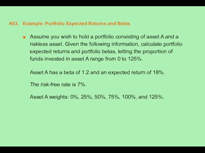
A53. Example: Portfolio Expected Returns and Betas
Assume you wish to hold
A53. Example: Portfolio Expected Returns and Betas
Assume you wish to hold
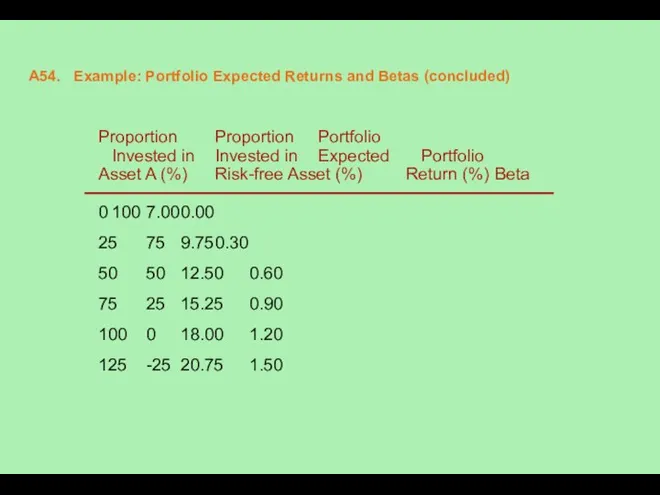
A54. Example: Portfolio Expected Returns and Betas (concluded)
Proportion Proportion Portfolio
Invested
A54. Example: Portfolio Expected Returns and Betas (concluded)
Proportion Proportion Portfolio Invested
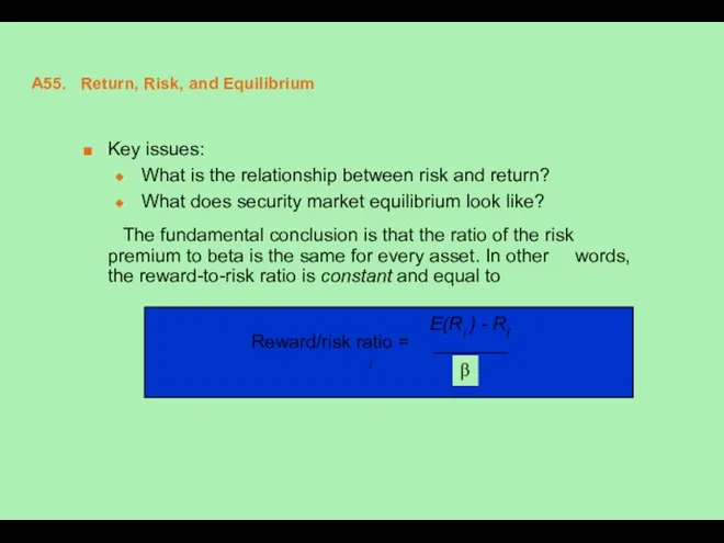
A55. Return, Risk, and Equilibrium
Key issues:
What is the relationship between risk
A55. Return, Risk, and Equilibrium
Key issues:
What is the relationship between risk
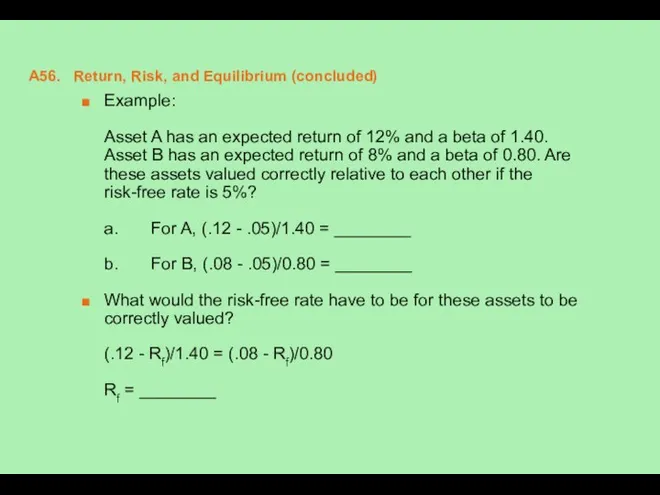
A56. Return, Risk, and Equilibrium (concluded)
Example:
Asset A has an expected
A56. Return, Risk, and Equilibrium (concluded)
Example:
Asset A has an expected
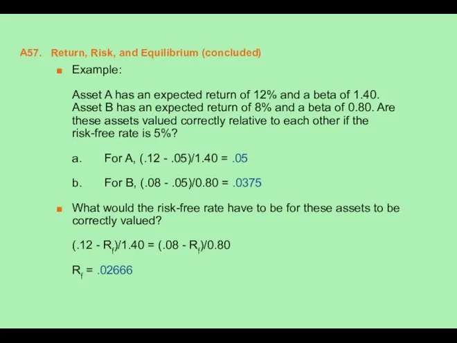
A57. Return, Risk, and Equilibrium (concluded)
Example:
Asset A has an expected
A57. Return, Risk, and Equilibrium (concluded)
Example:
Asset A has an expected
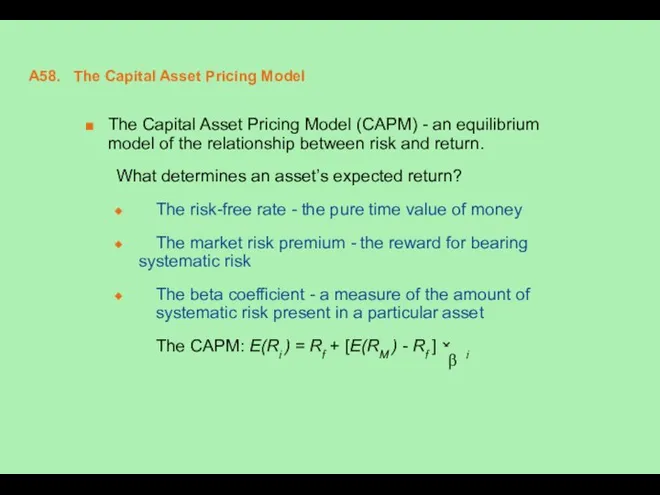
A58. The Capital Asset Pricing Model
The Capital Asset Pricing Model (CAPM)
A58. The Capital Asset Pricing Model
The Capital Asset Pricing Model (CAPM)
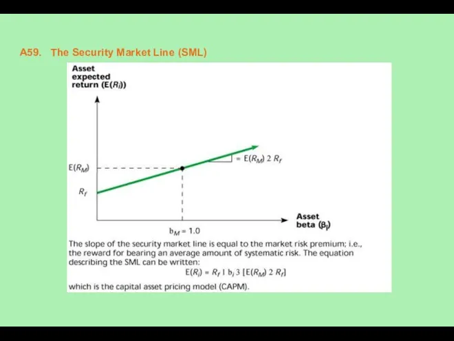
A59. The Security Market Line (SML)
A59. The Security Market Line (SML)
A60. Summary of Risk and Return
I. Total risk - the variance (or
A60. Summary of Risk and Return
I. Total risk - the variance (or
A61. Another Quick Quiz
1. Assume: the historic market risk premium has been
A61. Another Quick Quiz
1. Assume: the historic market risk premium has been
A62. Another Quick Quiz (continued)
1. Assume: the historic market risk premium has
A62. Another Quick Quiz (continued)
1. Assume: the historic market risk premium has
A63. An Example
Consider the following information:
State of Prob. of State Stock A Stock
A63. An Example
Consider the following information:
State of Prob. of State Stock A Stock
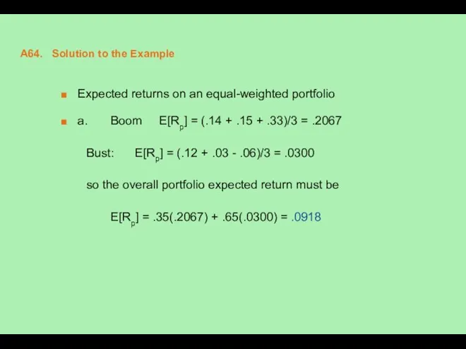
A64. Solution to the Example
Expected returns on an equal-weighted portfolio
a. Boom E[Rp] =
A64. Solution to the Example
Expected returns on an equal-weighted portfolio
a. Boom E[Rp] =
![A65. Solution to the Example (continued) b. Boom: E[Rp] =](/_ipx/f_webp&q_80&fit_contain&s_1440x1080/imagesDir/jpg/359583/slide-64.jpg)
A65. Solution to the Example (continued)
b. Boom: E[Rp] = __ (.14) + .15(.15)
A65. Solution to the Example (continued)
b. Boom: E[Rp] = __ (.14) + .15(.15)
![A66. Solution to the Example (concluded) b. Boom: E[Rp] =](/_ipx/f_webp&q_80&fit_contain&s_1440x1080/imagesDir/jpg/359583/slide-65.jpg)
A66. Solution to the Example (concluded)
b. Boom: E[Rp] = .15(.14) + .15(.15) +
A66. Solution to the Example (concluded)
b. Boom: E[Rp] = .15(.14) + .15(.15) +
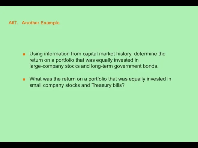
A67. Another Example
Using information from capital market history, determine the return
A67. Another Example
Using information from capital market history, determine the return
 Выпускная работа. Обоснование перспектив развития предприятия Фортуна Крым Трейд
 Ценообразование на монополизированном рынке
 Безработица. Трудоспособное и нетрудоспособное население
 Методы ABC, XYZ. Задача на знание метода ABC
 Макроэкономика. Сущность макроэкономики, ее основные цели
 Економічна теорія як наука
 Государственные финансы
 Märkte für Produktionsfaktoren
 Общая характеристика направления менеджмент и ее профилей. (Раздел 1)
 Денежно-кредитная политика государства
 Трудовые ресурсы предприятия: основные понятия, структура, показатели
 Организация и проведение массовой оценки объектов недвижимости
 Interaction of logical and nominal meanings
 Научно-техническая безопасность и экономический рост
 Теоретичні засади податків
 Собственность. Предпринимательство. Издержки производства. Прибыль
 Контроль за соблюдением норм и правил охраны труда. (Лекция 2)
 Задачи по экономике
 Экономическая природа фирмы: основные формы деловых предприятий
 Нематериальные активы (НМА) организации
 Экономика. Главные вопросы экономики
 Нобелевские премии по экономике
 Введение в логистику
 Основные производственные фонды. Понятие и классификация основных фондов
 Өндіріс факторларының арақатынасы теориясын эмпирикалық тексеру және олардың шектеулілігі мәселесі
 Неопределенность и риск в процессе реализации инвестиционных проектов
 Неолиберализм. Сущность и особенности неолиберализма
 Комплексный план развития Куединского муниципального округа Пермского края