- Demand assessment elementary methods

Содержание
- 2. 2 directions in demand assessment statistical analysis market intelligence Задача статистического анализа: определение параметров функции спроса
- 3. Statistical analysis Steps: 1) Collection, validation and assessment of data 2) The choice of the information
- 4. 1) Collection, validation and assessment of data time series cross-sectional data Statistical analysis
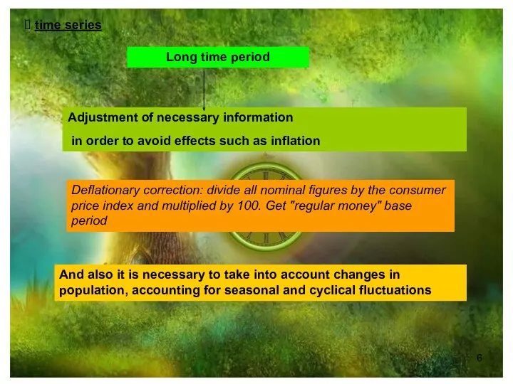
- 5. time series 1) Collection, validation and assessment of data Statistical analysis Examine time changes in the
- 6. Adjustment of necessary information in order to avoid effects such as inflation Deflationary correction: divide all
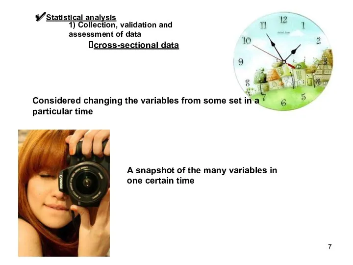
- 7. Statistical analysis 1) Collection, validation and assessment of data cross-sectional data Considered changing the variables from
- 8. Ex: In order to determine the effect of prices on demand, as a variable can be
- 9. Statistical analysis 2) The choice of the information curve The results of the observations are used
- 10. When choosing a curve there are two main questions: What type of equation it is necessary
- 11. If the trend of the experimental values of the dependent variable is approximately linear, and there
- 12. If the data can be reduced to a single independent variable (e.g. price) and the trend
- 13. If the trend of the dependent variable is nonlinear and the function has a single independent
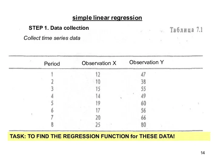
- 14. simple linear regression STEP 1. Data collection TASK: TO FIND THE REGRESSION FUNCTION for THESE DATA!
- 15. STEP 2. Organization variables in time simple linear regression Причины: визуализация; определение линейности или нелинейности для
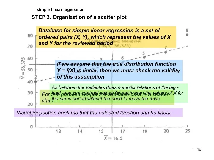
- 16. simple linear regression STEP 3. Organization of a scatter plot Database for simple linear regression is
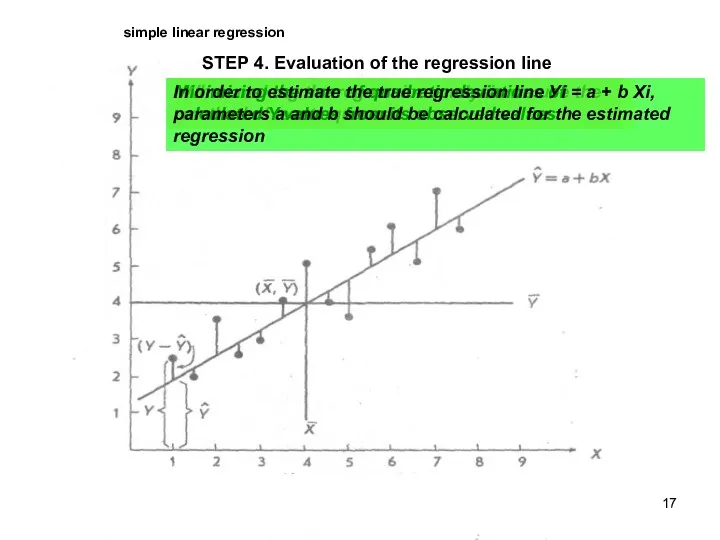
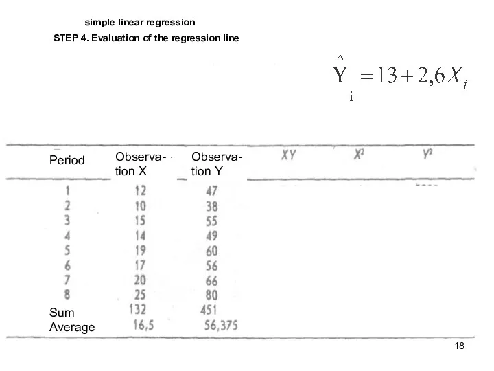
- 17. simple linear regression STEP 4. Evaluation of the regression line When making the regression analysis we
- 18. simple linear regression STEP 4. Evaluation of the regression line Period Observa-tion X Observa-tion X Observa-tion
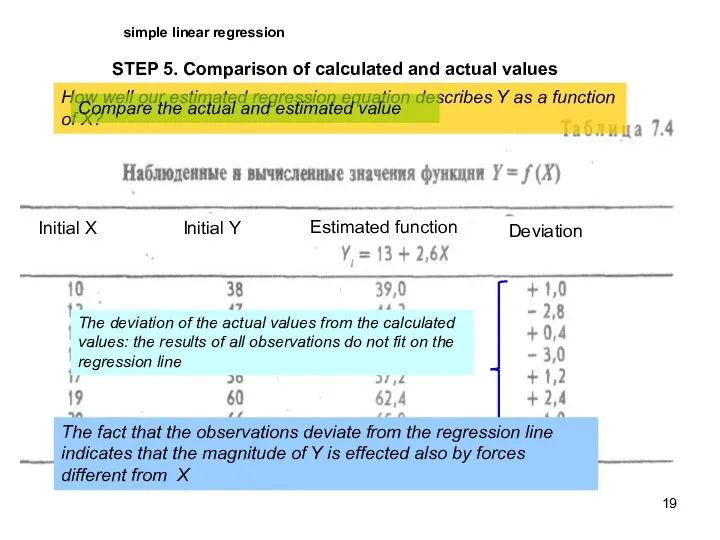
- 19. simple linear regression STEP 5. Comparison of calculated and actual values How well our estimated regression
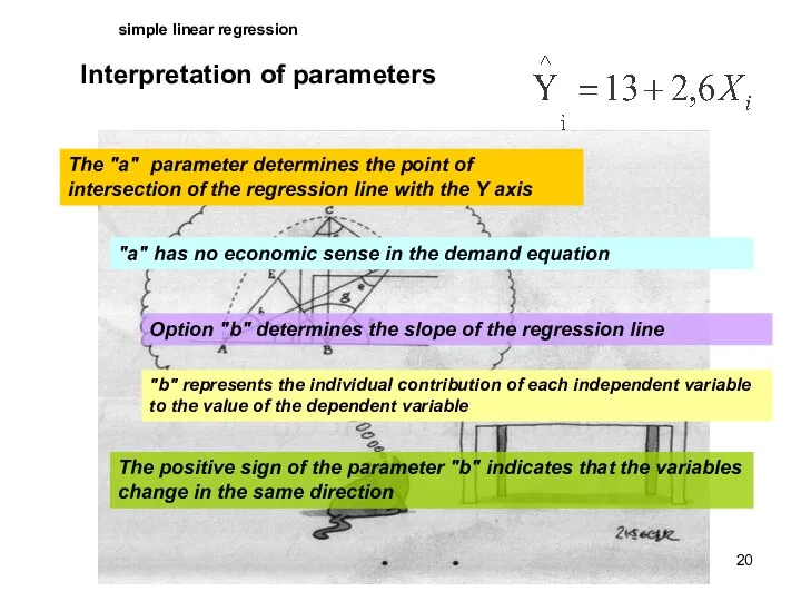
- 20. simple linear regression Interpretation of parameters The "a" parameter determines the point of intersection of the
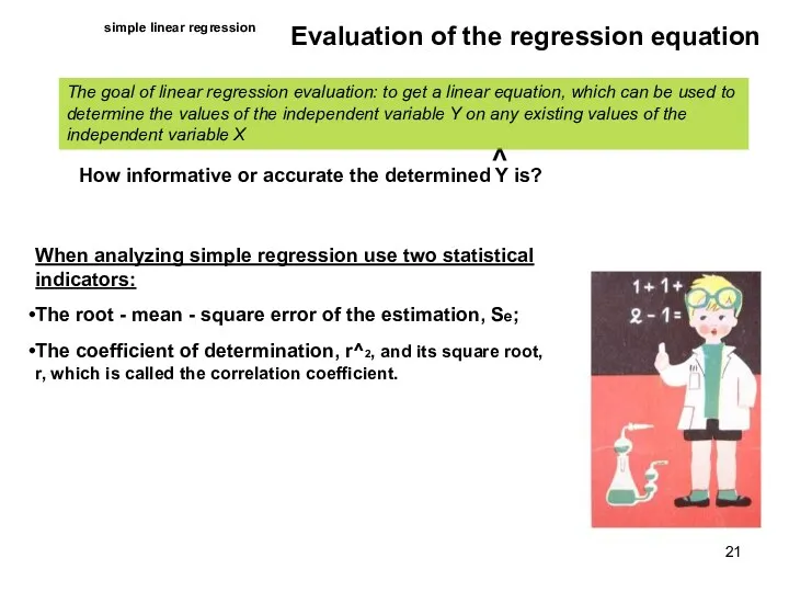
- 21. simple linear regression Evaluation of the regression equation How informative or accurate the determined Y is?
- 22. The root – mean - square error of the estimation, Se; Represents the deviation of experimental
- 23. The root - mean - square error of the estimation, Se; ˄ Root-mean-square error Observed Y
- 24. The more root-mean-square error is, the greater the range of deviations are Root-mean-square error, Se; If
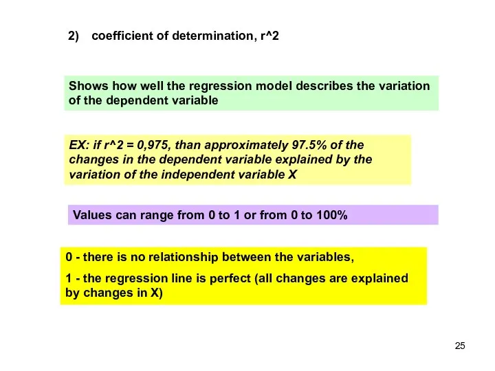
- 25. coefficient of determination, r^2 Shows how well the regression model describes the variation of the dependent
- 26. the correlation coefficient, r, Determines the degree of connection between variables -1 1
- 28. Скачать презентацию
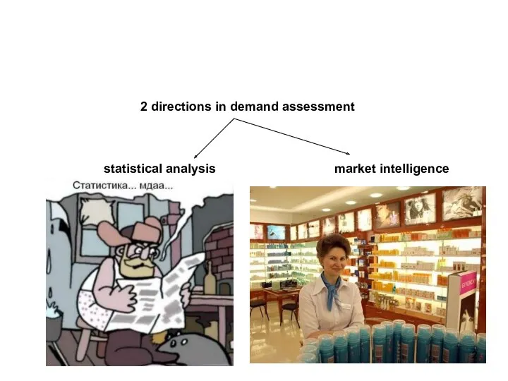
2 directions in demand assessment
statistical analysis
market intelligence
Задача статистического анализа: определение параметров
2 directions in demand assessment
statistical analysis
market intelligence
Задача статистического анализа: определение параметров
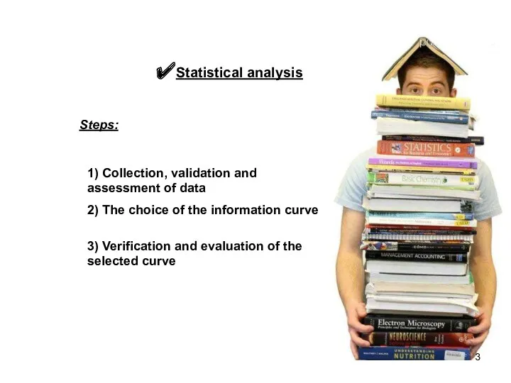
Statistical analysis
Steps:
1) Collection, validation and assessment of data
2) The choice of
Statistical analysis
Steps:
1) Collection, validation and assessment of data
2) The choice of
1) Collection, validation and assessment of data
time series
cross-sectional data
Statistical analysis
1) Collection, validation and assessment of data
time series
cross-sectional data
Statistical analysis
time series
1) Collection, validation and assessment of data
Statistical analysis
Examine time
time series
1) Collection, validation and assessment of data
Statistical analysis
Examine time
Adjustment of necessary information
in order to avoid effects such as
Adjustment of necessary information
in order to avoid effects such as
Statistical analysis
1) Collection, validation and assessment of data
cross-sectional data
Considered changing the
Statistical analysis
1) Collection, validation and assessment of data
cross-sectional data
Considered changing the
Ex: In order to determine the effect of prices on demand,
Ex: In order to determine the effect of prices on demand,
Statistical analysis
2) The choice of the information curve
The results of the
Statistical analysis
2) The choice of the information curve
The results of the
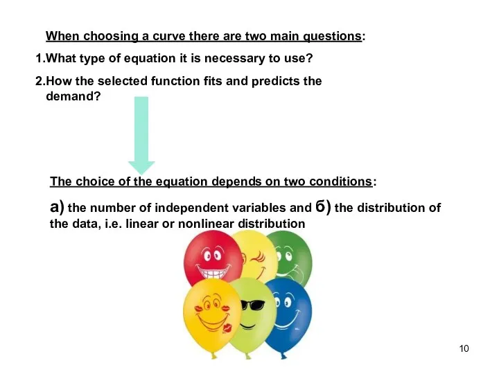
When choosing a curve there are two main questions:
What type of
When choosing a curve there are two main questions:
What type of
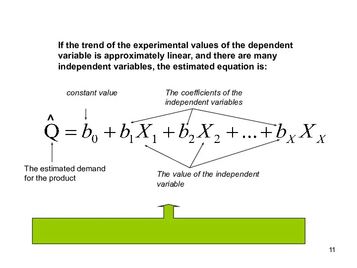
If the trend of the experimental values of the dependent variable
If the trend of the experimental values of the dependent variable
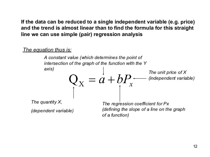
If the data can be reduced to a single independent variable
If the data can be reduced to a single independent variable
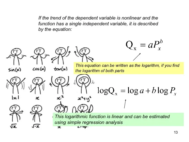
If the trend of the dependent variable is nonlinear and the
If the trend of the dependent variable is nonlinear and the
simple linear regression
STEP 1. Data collection
TASK: TO FIND THE REGRESSION FUNCTION
simple linear regression
STEP 1. Data collection
TASK: TO FIND THE REGRESSION FUNCTION
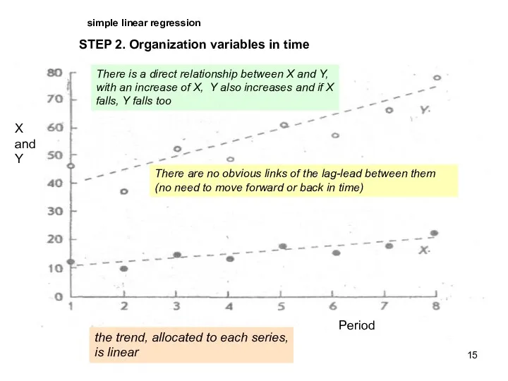
STEP 2. Organization variables in time
simple linear regression
Причины: визуализация; определение линейности
STEP 2. Organization variables in time
simple linear regression
Причины: визуализация; определение линейности
simple linear regression
STEP 3. Organization of a scatter plot
Database for simple
simple linear regression
STEP 3. Organization of a scatter plot
Database for simple
simple linear regression
STEP 4. Evaluation of the regression line
When making the
simple linear regression
STEP 4. Evaluation of the regression line
When making the
simple linear regression
STEP 4. Evaluation of the regression line
Period
Observa-tion X
Observa-tion X
Observa-tion
simple linear regression
STEP 4. Evaluation of the regression line
Period
Observa-tion X
Observa-tion X
Observa-tion
simple linear regression
STEP 5. Comparison of calculated and actual values
How well
simple linear regression
STEP 5. Comparison of calculated and actual values
How well
simple linear regression
Interpretation of parameters
The "a" parameter determines the point of
simple linear regression
Interpretation of parameters
The "a" parameter determines the point of
simple linear regression
Evaluation of the regression equation
How informative or accurate the
simple linear regression
Evaluation of the regression equation
How informative or accurate the
The root – mean - square error of the estimation, Se;
Represents
The root – mean - square error of the estimation, Se;
Represents
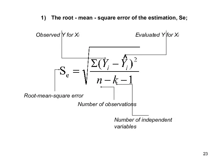
The root - mean - square error of the estimation, Se;
˄
Root-mean-square
The root - mean - square error of the estimation, Se;
˄
Root-mean-square
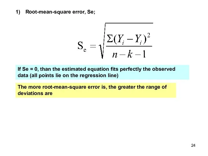
The more root-mean-square error is, the greater the range of deviations
The more root-mean-square error is, the greater the range of deviations
coefficient of determination, r^2
Shows how well the regression model describes the
coefficient of determination, r^2
Shows how well the regression model describes the
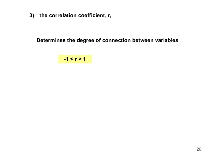
the correlation coefficient, r,
Determines the degree of connection between variables
-1
the correlation coefficient, r,
Determines the degree of connection between variables
-1
 Життя Вільяма Петті як основоположника класичної політичної економії в Англії в ХVII - ХVІІІ століттях
 Транспорттағы метеорологиялық болжамдардың экономикалық тиімділігі
 Общая характеристика рыночной экономики. (Тема 4)
 Развитие экономического сотрудничества в Евразии с участием России
 Коммерциализация технологий и разработок
 Анализ и диагностика финансово-хозяйственной деятельности предприятия. Экономический анализ
 Микроэкономика. Предмет и методология микроэкономики. Основные понятия
 Экономика и социология труда, как наука
 Определение оптимального объема производства: микроэкономический аспект
 Прогнозирование и планирование в условиях рынка
 Предмет и методы ЭТ. Базовые экономические категории. Лекция 1
 Сущность и задачи (экономическогО) районирования России
 Анализ производства и реализации продукции
 Оснвные средства предприятий
 Введение в микроэкономику
 Инновационная деятельность и повышение ее инвестиционной привлекательности
 International Economic. Analysis 1.1
 Фирменный стиль в рекламе
 Основные макроэкономические показатели
 Метод и методика экономического анализа
 Роль экономики в жизни общества
 Формування поведінки підприємства на ринку промислових товарів. (Тема 1)
 Экономические основы обеспечения безопасных условий труда. Методы управления охраной труда
 ARCH – модель та її практичне застосування в економіці
 Казахстанская модель экономического развития
 Основы антикризисного управления
 Понятие экономика
 Стратегия социально-экономического развития городского округа. Город Уфа Республики Башкортостан до 2030 года