- International Trade: Theory and Policy. Lecture 13

Содержание
- 2. Доклад ОЭСР «Health at a glance 2015»
- 3. Topics 9-11. International economic integration. International production factor migration. Lecture 13 International economic integration. International production
- 4. (9.1.) International economic integration Flam, H. (1992) Product markets and 1992: full integration, large gains? The
- 5. (9.1.) International economic integration ‘The goal of the 1992 program was to complete by January 1,
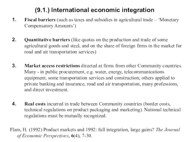
- 6. (9.1.) International economic integration Fiscal barriers (such as taxes and subsidies in agricultural trade – ‘Monetary
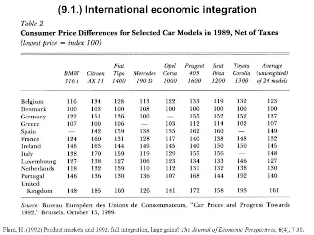
- 7. Flam, H. (1992) Product markets and 1992: full integration, large gains? The Journal of Economic Perspectives,
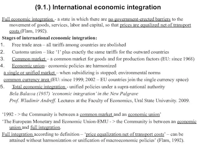
- 8. (9.1.) International economic integration Full economic integration - a state in which there are no government-erected
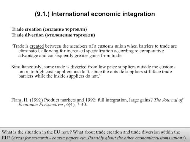
- 9. (9.1.) International economic integration Trade creation (создание торговли) Trade divertion (отклонение торговли) ‘Trade is created between
- 10. (9.1.) International economic integration Example. Eurasian Customs Union (Союз Россия-Беларусь-Казахстан). Advantages and challenges associated with customs
- 11. (9.2.) International production factor migration: theories and facts Labor Capital portfolio investment** foreign direct investment (FDI)
- 12. (9.2.) International production factor migration: theories and facts The gains-from-international factor migration theorem Graphical illustration: with
- 13. (9.2.) Structure of the model Structure of the world economy: 2 countries (h, f); One tradable
- 14. (9.2.) Revision: the gains-from-trade theorem The gains-from-trade theorem: Suppose that the value of production is maximized
- 15. (9.2.) International production factor migration: theories and facts The theorem on gains from international production factor
- 16. (9.2.) International production factor migration: theories and facts H-O-S model Based on the assumptions of H-O-S
- 17. (9.2.) Structure of the Heckscher-Ohlin-Samuelson (H-O-S) model of international trade Structure of the world economy :
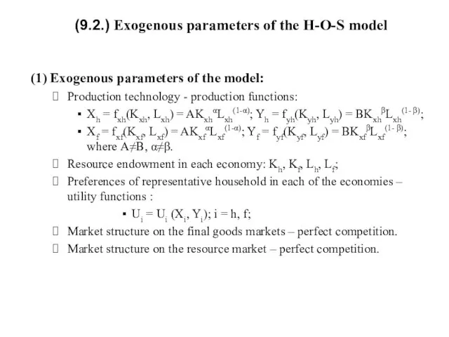
- 18. (9.2.) Exogenous parameters of the H-O-S model (1) Exogenous parameters of the model: Production technology -
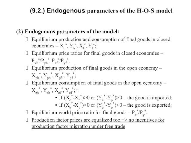
- 19. (9.2.) Endogenous parameters of the H-O-S model (2) Endogenous parameters of the model: Equilibrium production and
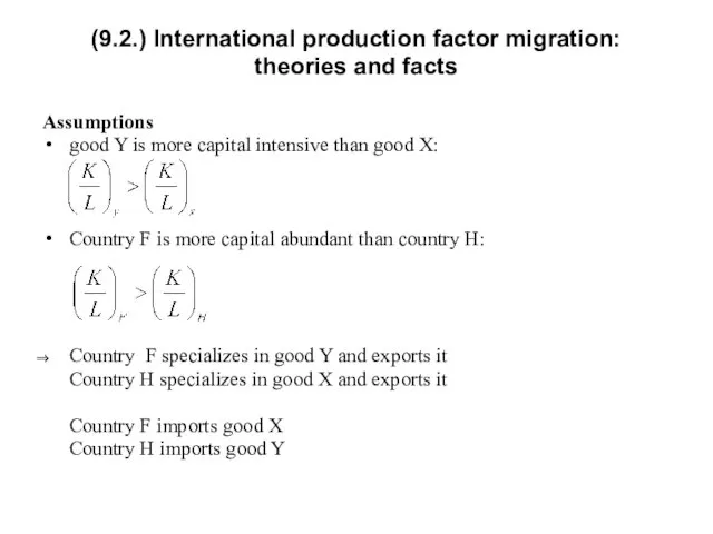
- 20. (9.2.) International production factor migration: theories and facts Assumptions good Y is more capital intensive than
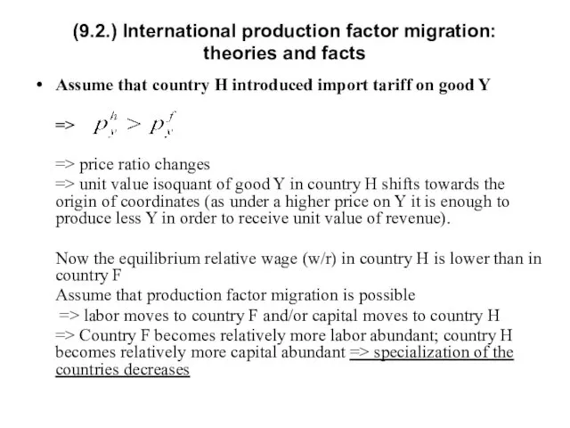
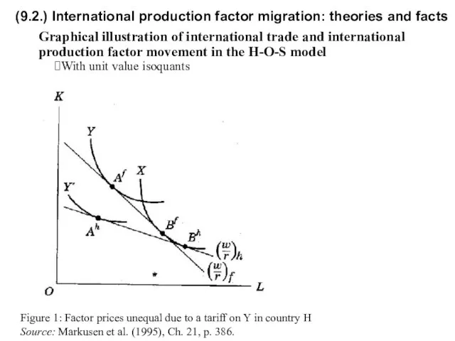
- 21. (9.2.) International production factor migration: theories and facts Assume that country Н introduced import tariff on
- 22. (9.2.) International production factor migration: theories and facts Graphical illustration of international trade and international production
- 23. (9.2.) International production factor migration: theories and facts Conclusions: In the H-O-S model the more production
- 24. (9.2.) International production factor migration: theories and facts D. Ricardo model Based on the assumptions of
- 25. (9.2.) Endogenous parameters of the modified Ricardian model (2 production factors) Structure of the world economy:
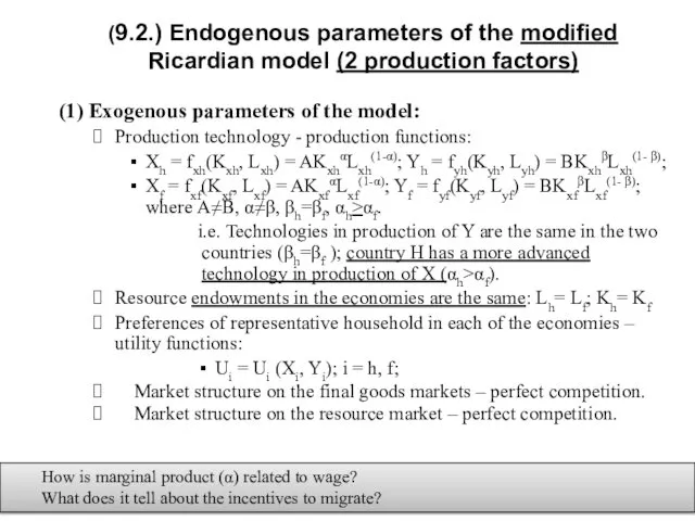
- 26. (9.2.) Endogenous parameters of the modified Ricardian model (2 production factors) (1) Exogenous parameters of the
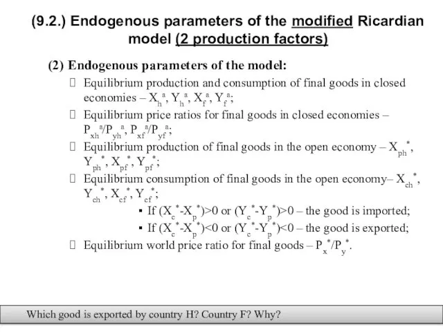
- 27. (9.2.) Endogenous parameters of the modified Ricardian model (2 production factors) (2) Endogenous parameters of the
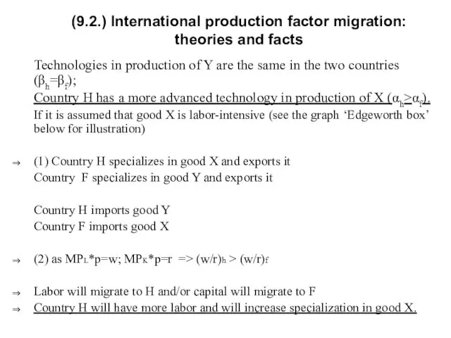
- 28. (9.2.) International production factor migration: theories and facts Technologies in production of Y are the same
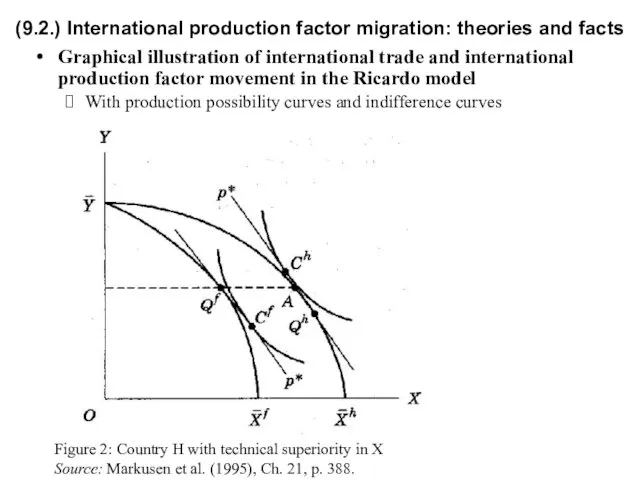
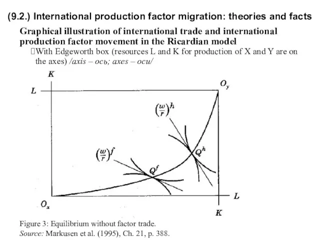
- 29. (9.2.) International production factor migration: theories and facts Graphical illustration of international trade and international production
- 30. (9.2.) International production factor migration: theories and facts Graphical illustration of international trade and international production
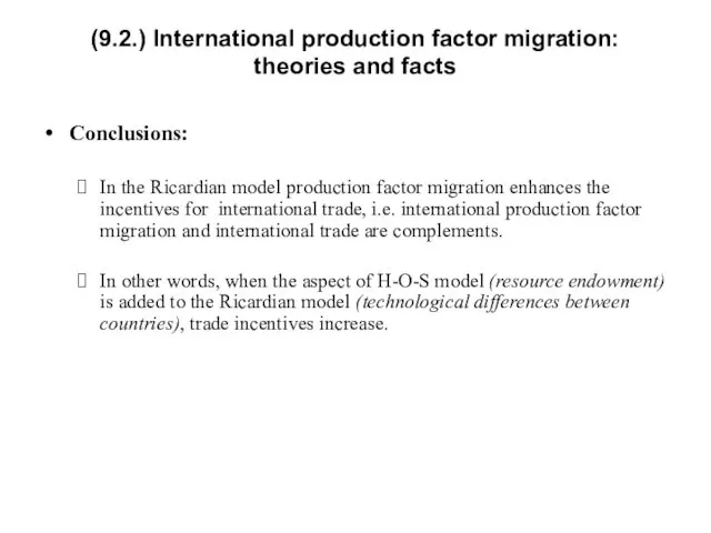
- 31. (9.2.) International production factor migration: theories and facts Conclusions: In the Ricardian model production factor migration
- 32. Exercise session 8 (2) Think about topics for reports during exercise sessions. (3) Start revising for
- 34. Скачать презентацию
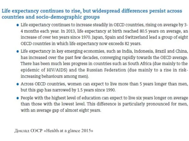
Доклад ОЭСР «Health at a glance 2015»
Доклад ОЭСР «Health at a glance 2015»
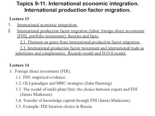
Topics 9-11. International economic integration. International production factor migration.
Lecture 13
International
Topics 9-11. International economic integration. International production factor migration.
Lecture 13
International
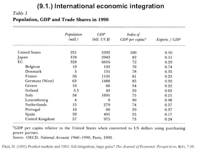
(9.1.) International economic integration
Flam, H. (1992) Product markets and 1992: full
(9.1.) International economic integration
Flam, H. (1992) Product markets and 1992: full
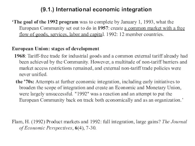
(9.1.) International economic integration
‘The goal of the 1992 program was to
(9.1.) International economic integration
‘The goal of the 1992 program was to
(9.1.) International economic integration
Fiscal barriers (such as taxes and subsidies in
(9.1.) International economic integration
Fiscal barriers (such as taxes and subsidies in
Flam, H. (1992) Product markets and 1992: full integration, large gains?
Flam, H. (1992) Product markets and 1992: full integration, large gains?
(9.1.) International economic integration
Full economic integration - a state in which
(9.1.) International economic integration
Full economic integration - a state in which
(9.1.) International economic integration
Trade creation (создание торговли)
Trade divertion (отклонение торговли)
‘Trade is
(9.1.) International economic integration
Trade creation (создание торговли)
Trade divertion (отклонение торговли)
‘Trade is
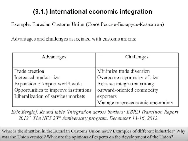
(9.1.) International economic integration
Example. Eurasian Customs Union (Союз Россия-Беларусь-Казахстан).
Advantages and challenges
(9.1.) International economic integration
Example. Eurasian Customs Union (Союз Россия-Беларусь-Казахстан).
Advantages and challenges
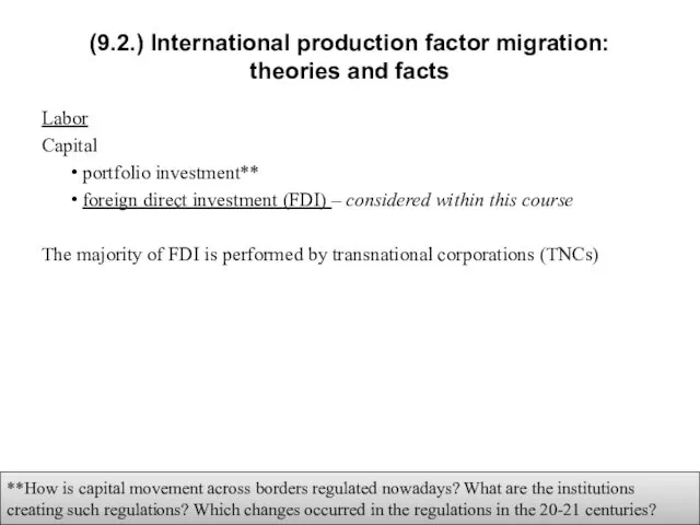
(9.2.) International production factor migration: theories and facts
Labor
Capital
portfolio investment**
foreign
(9.2.) International production factor migration: theories and facts
Labor
Capital
portfolio investment**
foreign
(9.2.) International production factor migration: theories and facts
The gains-from-international factor migration
(9.2.) International production factor migration: theories and facts
The gains-from-international factor migration
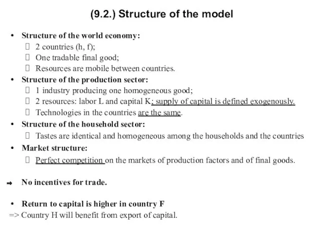
(9.2.) Structure of the model
Structure of the world economy:
2 countries (h,
(9.2.) Structure of the model
Structure of the world economy:
2 countries (h,
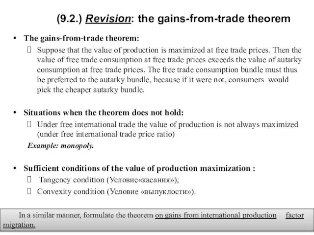
(9.2.) Revision: the gains-from-trade theorem
The gains-from-trade theorem:
Suppose that the value of
(9.2.) Revision: the gains-from-trade theorem
The gains-from-trade theorem:
Suppose that the value of
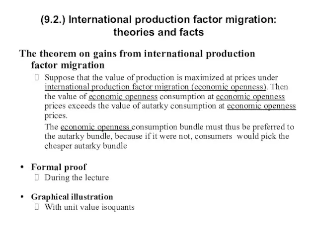
(9.2.) International production factor migration: theories and facts
The theorem on gains
(9.2.) International production factor migration: theories and facts
The theorem on gains
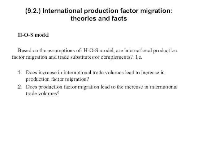
(9.2.) International production factor migration: theories and facts
H-O-S model
Based on the
(9.2.) International production factor migration: theories and facts
H-O-S model
Based on the
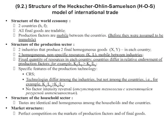
(9.2.) Structure of the Heckscher-Ohlin-Samuelson (H-O-S)
model of international trade
Structure of
(9.2.) Structure of the Heckscher-Ohlin-Samuelson (H-O-S)
model of international trade
Structure of
(9.2.) Exogenous parameters of the H-O-S model
(1) Exogenous parameters of the
(9.2.) Exogenous parameters of the H-O-S model
(1) Exogenous parameters of the
(9.2.) Endogenous parameters of the H-O-S model
(2) Endogenous parameters of
(9.2.) Endogenous parameters of the H-O-S model
(2) Endogenous parameters of
(9.2.) International production factor migration: theories and facts
Assumptions
good Y is
(9.2.) International production factor migration: theories and facts
Assumptions
good Y is
(9.2.) International production factor migration: theories and facts
Assume that country Н
(9.2.) International production factor migration: theories and facts
Assume that country Н
(9.2.) International production factor migration: theories and facts
Graphical illustration of international
(9.2.) International production factor migration: theories and facts
Graphical illustration of international
(9.2.) International production factor migration: theories and facts
Conclusions:
In the H-O-S model
(9.2.) International production factor migration: theories and facts
Conclusions:
In the H-O-S model
(9.2.) International production factor migration: theories and facts
D. Ricardo model
Based on
(9.2.) International production factor migration: theories and facts
D. Ricardo model
Based on
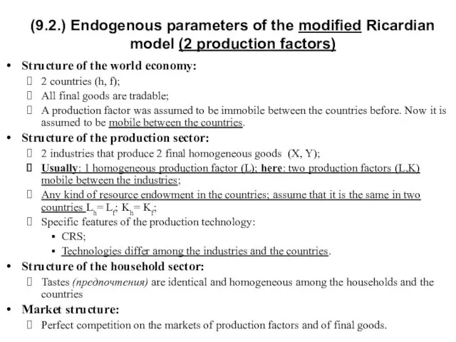
(9.2.) Endogenous parameters of the modified Ricardian model (2 production factors)
Structure
(9.2.) Endogenous parameters of the modified Ricardian model (2 production factors)
Structure
(9.2.) Endogenous parameters of the modified Ricardian model (2 production factors)
(1)
(9.2.) Endogenous parameters of the modified Ricardian model (2 production factors)
(1)
(9.2.) Endogenous parameters of the modified Ricardian model (2 production factors)
(2)
(9.2.) Endogenous parameters of the modified Ricardian model (2 production factors)
(2)
(9.2.) International production factor migration: theories and facts
Technologies in production
(9.2.) International production factor migration: theories and facts
Technologies in production
(9.2.) International production factor migration: theories and facts
Graphical illustration of international
(9.2.) International production factor migration: theories and facts
Graphical illustration of international
(9.2.) International production factor migration: theories and facts
Graphical illustration of international
(9.2.) International production factor migration: theories and facts
Graphical illustration of international
(9.2.) International production factor migration: theories and facts
Conclusions:
In the Ricardian model
(9.2.) International production factor migration: theories and facts
Conclusions:
In the Ricardian model
Exercise session 8
(2) Think about topics for reports during exercise sessions.
(3)
(2) Think about topics for reports during exercise sessions.
(3)
 Дүниежүзілік шаруашылықтың қалыптасуы және оның кұрылымы
 Энергосбытовая компания как агрегатор управления спросом
 Экономический рост и развитие
 Индикаторы устойчивого развития
 Изменения законодательства о применении контрольно-кассовой техники. Слайды для доклада Дронова И.В. 12.10.2016
 Производственные ресурсы предприятий НГК и эффективность их использования
 Теория экономического цикла (взгляд австрийской школы)
 Совершенная и несовершенная конкуренция. Монополия. Антимонопольная деятельность государства. (Тема 7-8)
 Indicators of economic development
 Кейс ХМАО-Югра. Точки роста для экономики региона
 Основные организационно-правовые формы предприятий
 Рынок труда. Специфика и объекты рынка труда. Функции, механизмы и особенности рынка труда
 Terms of Trade and Global Efficiency Effects of Free Trade Agreements
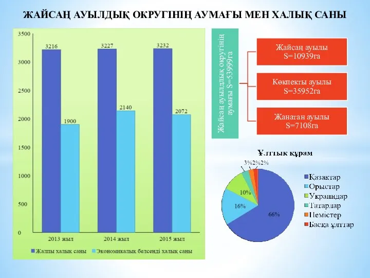 Саны экономикалық белсенді халық
 Экономика Китая
 Проблемы развивающегося мира
 Институциональная динамика
 Теория поведения потребителя
 Международные финансовые организации
 Сущность и функции предпринимательства
 Постсоветское пространство: Центральная Азия
 Макроэкономика. (Семинар 1)
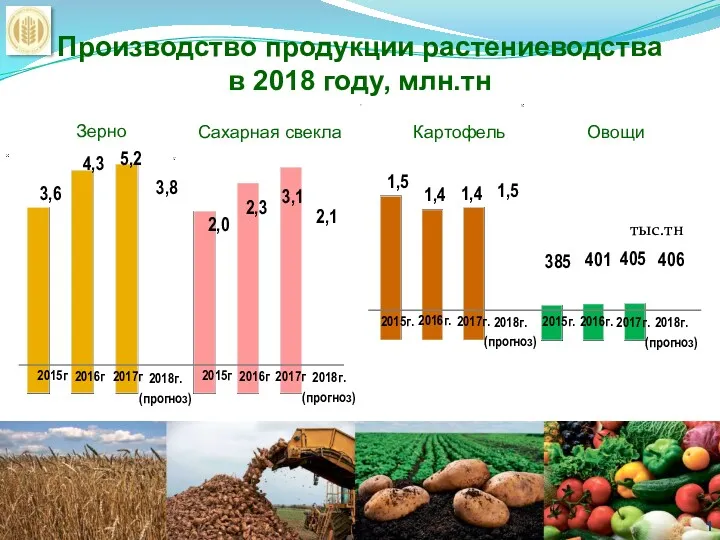 Производство продукции растениеводства в 2018 году, млн.тонн
 Рынок и рыночный механизм. Спрос и предложение
 Культура Германии
 Основний капітал підприємства. (Лекція 2)
 Показатели индустрии туризма. Австрия
 Безработица. Основные причины безработицы