- Model of aggregate demand and aggregate supply. Topic 3

Содержание
- 2. 1. Aggregate demand and its model. AD curve AGGREGATE DEMAND (AD) – is a schedule or
- 3. 1. Aggregate demand and its model. AD curve Aggregate demand is the planned expenditure in all
- 4. 1. Aggregate demand and its model. AD curve Because of the negative relationship between the level
- 5. 1. Aggregate demand and its model. AD curve AD factors are divided into: Price related –
- 6. 1. Aggregate demand and its model. AD curve Price related factors: 1. Real-Balances Effect (wealth effect)-
- 7. 1. Aggregate demand and its model. AD curve Price related factors: 2. Interest-Rate(Savings) Effect - with
- 8. 1. Aggregate demand and its model. AD curve 3. Foreign Purchases Effect - the increase in
- 9. NON PRICE RELATED FACTORS shift the aggregate demand curve. They are also known as Aggregate demand
- 10. 1. Aggregate demand and its model. AD curve 1. Change in consumer spending Consumer Wealth -
- 11. 1. Aggregate demand and its model. AD curve 1. Change in consumer spending Consumer Expectations .When
- 12. 1. Aggregate demand and its model. AD curve 2. Investment Spending Real Interest Rates Other things
- 13. 1. Aggregate demand and its model. AD curve Expected returns, in turn, are influenced by several
- 14. 1. Aggregate demand and its model. AD curve 3. Government Spending An increase in government purchases
- 15. 1. Aggregate demand and its model. AD curve 4. Net Export Spending Other things equal, higher
- 16. 1. Aggregate demand and its model. AD curve Causes of net exports change: National Income Abroad
- 17. 2. Aggregate supply in the short and long run. Factors affecting the aggregate supply. AS curve.
- 18. 2. Aggregate supply in the short and long run. Factors affecting the aggregate supply. AS curve.
- 19. АS Shifters or non-price related factors of AS.
- 20. 2. Aggregate supply in the short and long run. Factors affecting the aggregate supply. AS curve.
- 21. 2. Aggregate supply in the short and long run. Factors affecting the aggregate supply. AS curve.
- 22. 2. Aggregate supply in the short and long run. Factors affecting the aggregate supply. AS curve.
- 23. 2. Aggregate supply in the short and long run. Factors affecting the aggregate supply. AS curve.
- 24. The shape of the AS curve is interpreted differently in Classical and Keynesian theories. Classical theory
- 25. 2. Aggregate supply in the short and long run. Factors affecting the aggregate supply. AS curve.
- 26. 2. Aggregate supply in the short and long run. Factors affecting the aggregate supply. AS curve.
- 27. 2. Aggregate supply in the short and long run. Factors affecting the aggregate supply. AS curve.
- 28. 2. Aggregate supply in the short and long run. Factors affecting the aggregate supply. AS curve.
- 29. 2. Aggregate supply in the short and long run. Factors affecting the aggregate supply. AS curve.
- 30. 3. Macroeconomic equilibrium in AD-AS model. At the point of intersection of the curves of aggregate
- 31. 3. Macroeconomic equilibrium in AD-AS model.
- 32. Variants of macroeconomic equilibrium
- 33. Variants of macroeconomic equilibrium If aggregate demand changes within the Keynesian segment, then the growth of
- 35. Скачать презентацию
 Основные определения, принятые в международной практике внешней торговли
 Российский рынок систем умного дома
 Господарство первісного суспільства та його еволюція на етапі ранніх цивілізацій
 Урок экономики по теме: Организационно-правовые формы предпринимательства
 Рынки факторов производства
 Ограниченность возможностей рынка. Смешанная экономика
 Московская служба занятости
 Экспорт и импорт в Казахстане
 Социально-экономическая организация
 Нетрадиционные системы оплаты труда. Вопрос 7
 Фирмы в экономике, или КАК разбогатеть
 Финансово-экономические характеристики деятельности публичных компаний
 Экономические взгляды Карла Маркса и Фридриха Энгельса
 Регулирование социального развития и уровня жизни населения
 Manufacturing Statistics Current trends and challenges
 Экономические основы деятельности фирмы
 Взаимодействие спроса и предложения
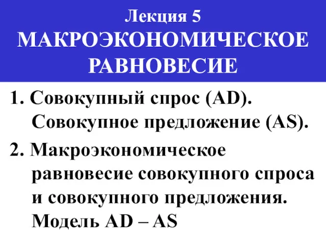 Совокупный спрос (AD). Совокупное предложение (AS). Макроэкономическое равновесие совокупного спроса и совокупного предложения
 В поисках решения проблем глобальной безопасности
 Анализ подходов к формированию финансовой политики предприятий лесоперерабатывающей отрасли в условиях эконом. нестабильности
 Понятие и состав основных фондов организации (предприятия)
 Факторы, влияющие на потребность организации в персонале
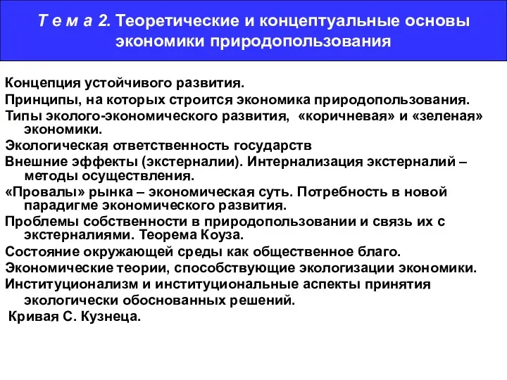 Теоретические и концептуальные основы экономики природопользования (Тема 2)
 Теория спроса и предложения
 Бедность и её оценка
 Единое экономическое пространство
 Роль олигополии в российской экономике
 Что такое экономика