- National Income: Where It Comes From and Where It Goes

Содержание
- 2. IN THIS CHAPTER, YOU WILL LEARN: What determines the economy’s total output/ income How the prices
- 3. Outline of model CHAPTER 3 National Income 2 A closed economy, market-clearing model Supply side factor
- 4. Factors of production CHAPTER 3 National Income 3 K = capital: tools, machines, and structures used
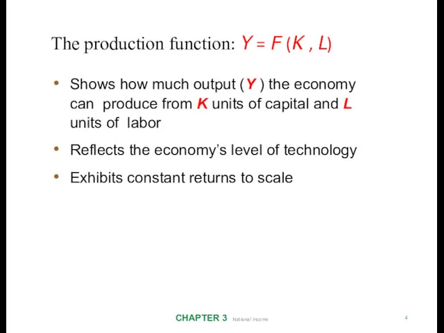
- 5. The production function: Y = F (K , L) CHAPTER 3 National Income 4 Shows how
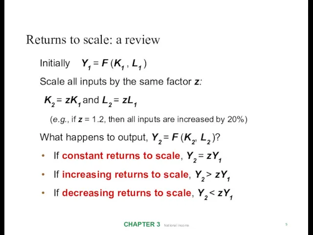
- 6. Returns to scale: a review CHAPTER 3 National Income 5 Initially Y1 = F (K1 ,
- 7. Returns to scale: Example 1 CHAPTER 3 National Income 6 KL (zK)(zL) F(K,L) = F(zK,zL) =
- 8. Returns to scale: Example 2 CHAPTER 3 National Income 7 F(K,L) = K 2 + L2
- 9. NOW YOU TRY 8 Determine whether each of these production functions has constant, decreasing, or increasing
- 10. NOW YOU TRY 9 L F (K,L) = K 2 zL F (zK, zL) = (zK
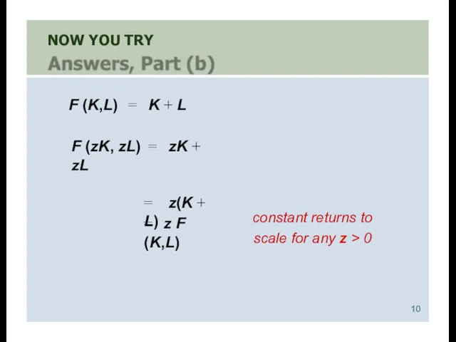
- 11. NOW YOU TRY F (K,L) = K + L F (zK, zL) = zK + zL
- 12. Assumptions CHAPTER 3 National Income 11 Technology is fixed. The economy’s supplies of capital and labor
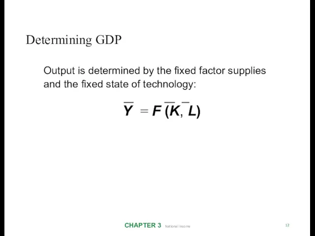
- 13. Determining GDP CHAPTER 3 National Income 12 Output is determined by the fixed factor supplies and
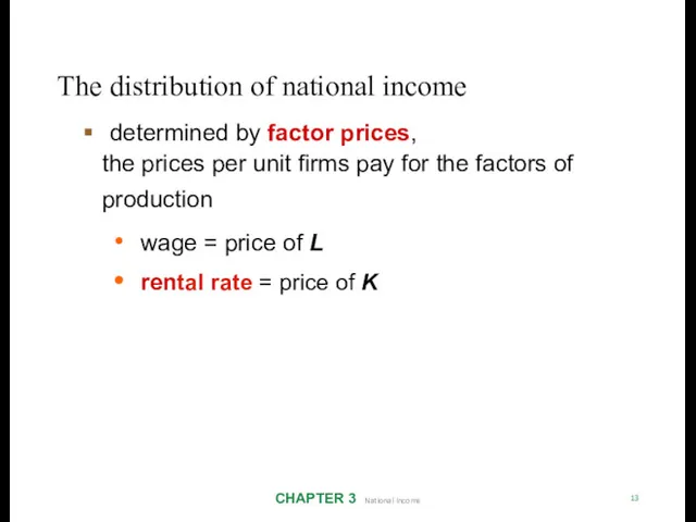
- 14. The distribution of national income CHAPTER 3 National Income 13 determined by factor prices, the prices
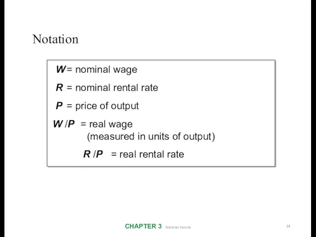
- 15. Notation CHAPTER 3 National Income 14 W = nominal wage R = nominal rental rate P
- 16. How factor prices are determined CHAPTER 3 National Income 15 Factor prices are determined by supply
- 17. Demand for labor CHAPTER 3 National Income 16 Assume markets are competitive: each firm takes W,
- 18. Marginal product of labor (MPL ) CHAPTER 3 National Income 17 Definition: The extra output the
- 19. NOW YOU TRY Compute & graph MPL 18 Determine MPL at each value of L. Graph
- 20. ANSWERS Compute & graph MPL 19 MPL (units of output) Marginal Product of Labor 12 10
- 21. Y output MPL and the production function CHAPTER 3 National Income 20 L labor F (K
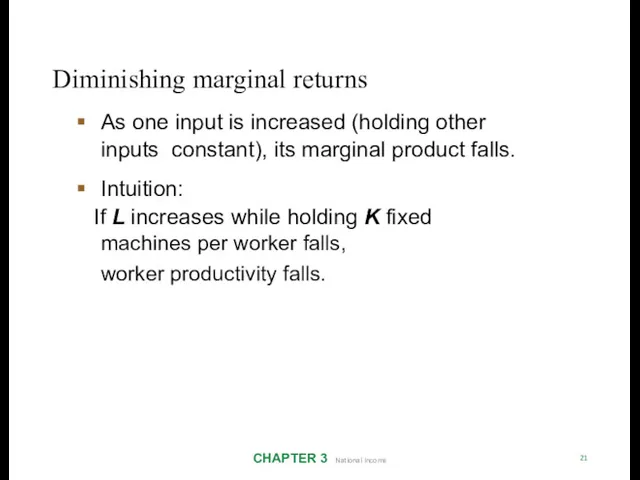
- 22. Diminishing marginal returns CHAPTER 3 National Income 21 As one input is increased (holding other inputs
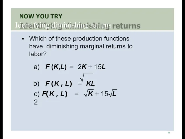
- 23. NOW YOU TRY Identifying diminishing returns 22 Which of these production functions have diminishing marginal returns
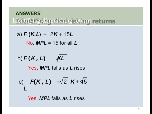
- 24. ANSWERS Identifying diminishing returns 23 a) F (K,L) = 2K + 15L No, MPL = 15
- 25. 24
- 26. worker adds MPL = 4 units of output 25
- 27. MPL and the demand for labor CHAPTER 3 National Income 26 Each firm hires labor up
- 28. The equilibrium real wage CHAPTER 3 National Income 27 The real wage adjusts to equate labor
- 29. Determining the rental rate CHAPTER 3 National Income 28 We have just seen that MPL =
- 30. The equilibrium real rental rate CHAPTER 3 National Income 29 The real rental rate adjusts to
- 31. The neoclassical theory of distribution CHAPTER 3 National Income 30 States that each factor input is
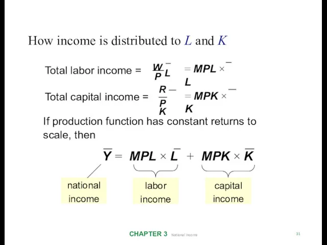
- 32. How income is distributed to L and K CHAPTER 3 National Income 31 Total labor income
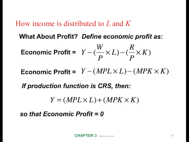
- 33. How income is distributed to L and K CHAPTER 3 National Income 32
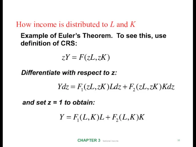
- 34. How income is distributed to L and K CHAPTER 3 National Income 33
- 35. How income is distributed to L and K CHAPTER 3 National Income 34
- 36. 0.1 0 0.2 0.3 0.4 0.7 0.6 0.5 0.8 0.9 1 1960 1965 1970 1975 1980
- 37. The Cobb-Douglas production function has constant factor shares: CHAPTER 3 National Income 36 The Cobb-Douglas production
- 38. The Cobb-Douglas production function CHAPTER 3 National Income 37 Each factor’s marginal product is proportional to
- 39. Labor productivity and wages CHAPTER 3 National Income 38 Theory: wages depend on labor productivity U.S.
- 40. The growing gap between rich & poor 0.30 0.45 0.50 0.40 Gini coefficient 0.35 Inequality has
- 41. Explanations for rising inequality CHAPTER 3 National Income 40 Rise in capital’s share of income, since
- 42. Outline of model CHAPTER 3 National Income 41 A closed economy, market-clearing model Supply side DONE
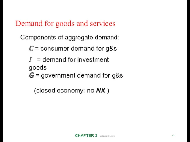
- 43. Demand for goods and services CHAPTER 3 National Income 42 Components of aggregate demand: C =
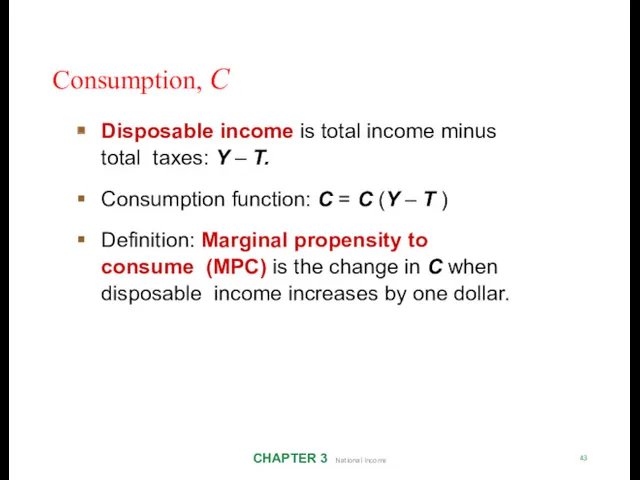
- 44. Consumption, C CHAPTER 3 National Income 43 Disposable income is total income minus total taxes: Y
- 45. The consumption function CHAPTER 3 National Income 44 C Y – T C (Y –T )
- 46. Investment, I CHAPTER 3 National Income 45 The investment function is I = I (r )
- 47. The investment function CHAPTER 3 National Income 46 r I (r ) I Spending on investment
- 48. Government spending, G CHAPTER 3 National Income 47 G = govt spending on goods and services
- 49. The market for goods & services CHAPTER 3 National Income 48 Aggregate demand: Aggregate supply: Equilibrium:
- 50. The loanable funds market CHAPTER 3 National Income 49 A simple supply–demand model of the financial
- 51. Demand for funds: investment CHAPTER 3 National Income 50 The demand for loanable funds . .
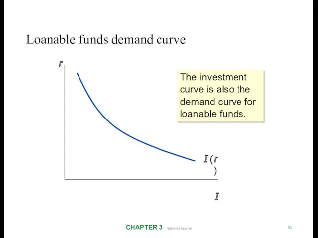
- 52. Loanable funds demand curve CHAPTER 3 National Income 51 r I (r ) I The investment
- 53. Supply of funds: saving CHAPTER 3 National Income 52 The supply of loanable funds comes from
- 54. Types of saving CHAPTER 3 National Income 53 Private saving Public saving = (Y – T
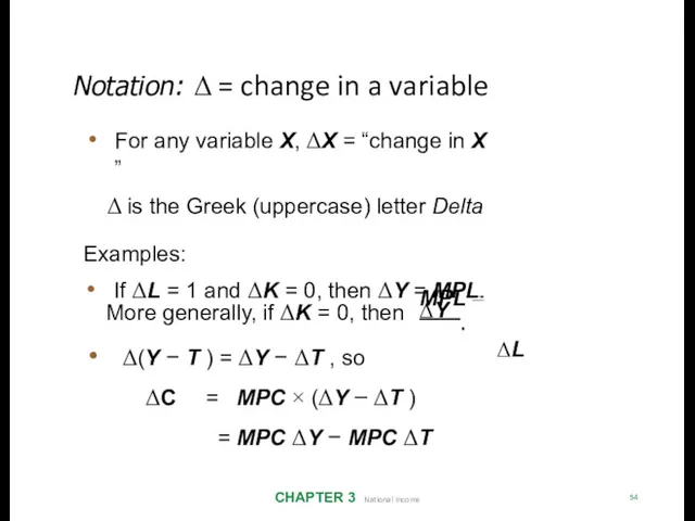
- 55. Notation: Δ = change in a variable CHAPTER 3 National Income 54 For any variable X,
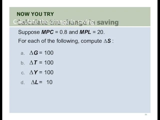
- 56. NOW YOU TRY Calculate the change in saving 55 Suppose MPC = 0.8 and MPL =
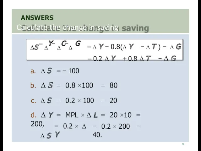
- 57. ANSWERS Calculate the change in saving 56 ΔS = ΔY− ΔC−Δ G = Δ Y −
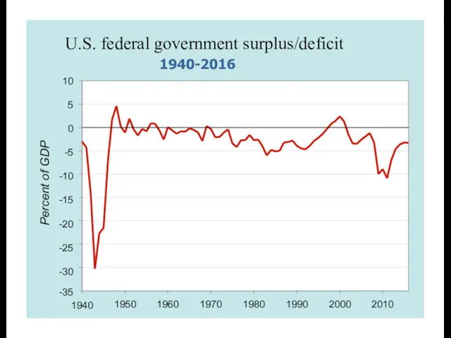
- 58. 57 CHAPTER 3 National Income Budget surpluses and deficits If T > G, budget surplus If
- 59. 1940-2016 Percent of GDP 10 5 0 -5 -10 -15 -20 -25 -30 -35 1940 1950
- 60. U.S. federal government debt, 1940-2016 Percent of GDP 140 120 100 80 60 40 20 0
- 61. Loanable funds supply curve CHAPTER 3 National Income 60 r S, I S =Y − C
- 62. Loanable funds market equilibrium CHAPTER 3 National Income 61 r S, I I (r ) S
- 63. The special role of r CHAPTER 3 National Income 62 r adjusts to equilibrate the goods
- 64. Digression: mastering models CHAPTER 3 National Income 63 To master a model, be sure to know:
- 65. Mastering the loanable funds model CHAPTER 3 National Income 64 Things that shift the saving curve:
- 66. CASE STUDY: The Reagan Deficits CHAPTER 3 National Income 65 Reagan policies during early 1980s: increases
- 67. CASE STUDY: The Reagan Deficits CHAPTER 3 National Income 66 r S, I S 1 I
- 68. Are the data consistent with these results? CHAPTER 3 National Income 67 T–G, S, and I
- 69. NOW YOU TRY 68 Draw the diagram for the loanable funds model. Suppose the tax laws
- 70. Mastering the loanable funds model CHAPTER 3 National Income 69 (continued) Things that shift the investment
- 71. An increase in investment demand CHAPTER 3 National Income 79 An increase in desired investment… r
- 72. Saving and the interest rate CHAPTER 3 National Income 71 Why might saving depend on r
- 73. An increase in investment demand when saving depends on r CHAPTER 3 National Income 72 r
- 74. C H A P T E R S U M M A R Y Total output
- 75. C H A P T E R S U M M A R Y A closed
- 77. Скачать презентацию
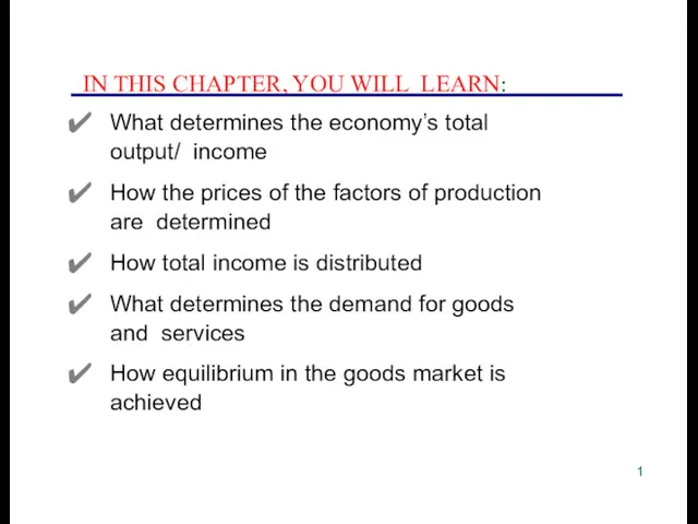
IN THIS CHAPTER, YOU WILL LEARN:
What determines the economy’s total output/
IN THIS CHAPTER, YOU WILL LEARN:
What determines the economy’s total output/
Outline of model
CHAPTER 3 National Income
2
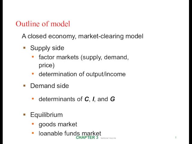
A closed economy, market-clearing model
Supply side
factor
Outline of model
CHAPTER 3 National Income
2
A closed economy, market-clearing model
Supply side
factor

Factors of production
CHAPTER 3 National Income
3
K = capital:
tools, machines, and structures used
Factors of production
CHAPTER 3 National Income
3
K = capital:
tools, machines, and structures used
The production function: Y = F (K , L)
CHAPTER 3 National
The production function: Y = F (K , L)
CHAPTER 3 National
Returns to scale: a review
CHAPTER 3 National Income
5
Initially Y1 = F (K1
Returns to scale: a review
CHAPTER 3 National Income
5
Initially Y1 = F (K1
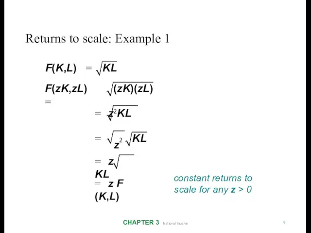
Returns to scale: Example 1
CHAPTER 3 National Income
6
KL
(zK)(zL)
F(K,L) =
F(zK,zL) =
= z2KL
KL
=
z2
= z KL
= z F (K,L)
constant returns
Returns to scale: Example 1
CHAPTER 3 National Income
6
KL
(zK)(zL)
F(K,L) =
F(zK,zL) =
= z2KL
KL
=
z2
= z KL
= z F (K,L)
constant returns
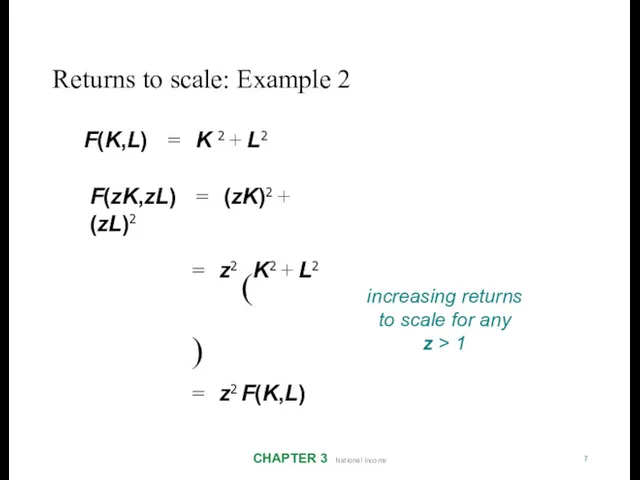
Returns to scale: Example 2
CHAPTER 3 National Income
7
F(K,L) = K 2 + L2
F(zK,zL) = (zK)2
Returns to scale: Example 2
CHAPTER 3 National Income
7
F(K,L) = K 2 + L2
F(zK,zL) = (zK)2
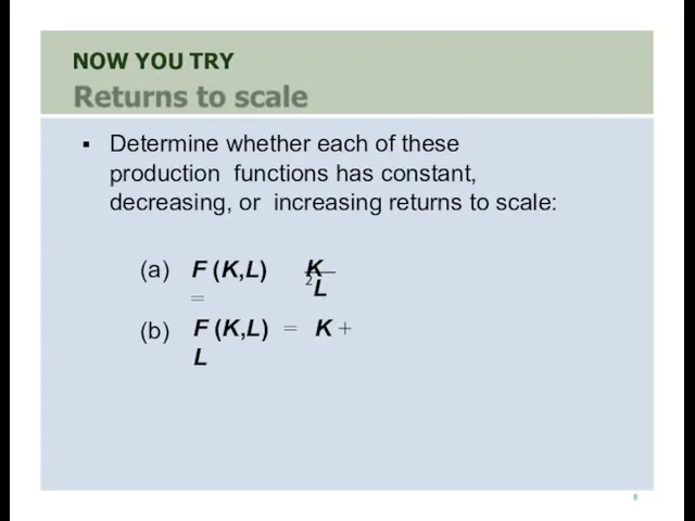
NOW YOU TRY
8
Determine whether each of these production functions has constant,
NOW YOU TRY
8
Determine whether each of these production functions has constant,
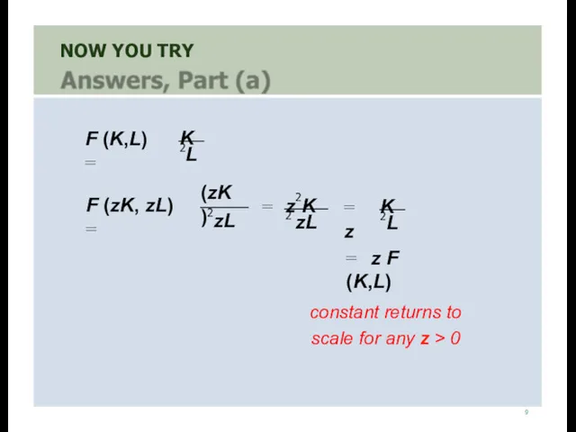
NOW YOU TRY
9
L
F (K,L) =
K 2
zL
F (zK, zL) =
(zK )2
zL
=
z2K 2
L
= z
K 2
= z F
NOW YOU TRY
9
L
F (K,L) =
K 2
zL
F (zK, zL) =
(zK )2
zL
=
z2K 2
L
= z
K 2
= z F
NOW YOU TRY
F (K,L) = K + L
F (zK, zL) = zK + zL
= z(K +
NOW YOU TRY
F (K,L) = K + L
F (zK, zL) = zK + zL
= z(K +

Assumptions
CHAPTER 3 National Income
11
Technology is fixed.
The economy’s supplies of capital and
Assumptions
CHAPTER 3 National Income
11
Technology is fixed.
The economy’s supplies of capital and
Determining GDP
CHAPTER 3 National Income
12
Output is determined by the fixed factor
Determining GDP
CHAPTER 3 National Income
12
Output is determined by the fixed factor
The distribution of national income
CHAPTER 3 National Income
13
determined by factor prices,
the
The distribution of national income
CHAPTER 3 National Income
13
determined by factor prices,
the
Notation
CHAPTER 3 National Income
14
W = nominal wage
R = nominal rental rate
P = price of
Notation
CHAPTER 3 National Income
14
W = nominal wage
R = nominal rental rate
P = price of

How factor prices are determined
CHAPTER 3 National Income
15
Factor prices are determined
How factor prices are determined
CHAPTER 3 National Income
15
Factor prices are determined

Demand for labor
CHAPTER 3 National Income
16
Assume markets are competitive: each firm
Demand for labor
CHAPTER 3 National Income
16
Assume markets are competitive: each firm
Marginal product of labor (MPL )
CHAPTER 3 National Income
17
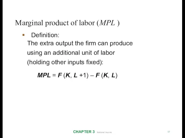
Definition:
The extra
Marginal product of labor (MPL )
CHAPTER 3 National Income
17
Definition:
The extra
NOW YOU TRY
Compute & graph MPL
18
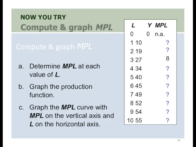
Determine MPL at each value of
NOW YOU TRY
Compute & graph MPL
18
Determine MPL at each value of
ANSWERS
Compute & graph MPL
19
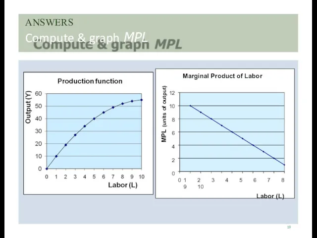
MPL (units of output)
Marginal Product of Labor
12
10
8
6
4
2
0
0 1 2 3 4 5 6 7 8 9 10
Labor (L)
ANSWERS
Compute & graph MPL
19
MPL (units of output)
Marginal Product of Labor
12
10
8
6
4
2
0
0 1 2 3 4 5 6 7 8 9 10
Labor (L)
Y
output
MPL and the production function
CHAPTER 3 National Income
20
L
labor
F (K , L)
1
MPL
1
MPL
1
MPL
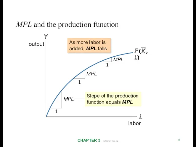
As
Y
output
MPL and the production function
CHAPTER 3 National Income
20
L
labor
F (K , L)
1
MPL
1
MPL
1
MPL
As
Diminishing marginal returns
CHAPTER 3 National Income
21
As one input is increased (holding
Diminishing marginal returns
CHAPTER 3 National Income
21
As one input is increased (holding
NOW YOU TRY
Identifying diminishing returns
22
Which of these production functions have diminishing
NOW YOU TRY
Identifying diminishing returns
22
Which of these production functions have diminishing
ANSWERS
Identifying diminishing returns
23
a) F (K,L) = 2K + 15L
No, MPL = 15 for all
ANSWERS
Identifying diminishing returns
23
a) F (K,L) = 2K + 15L
No, MPL = 15 for all
24
24
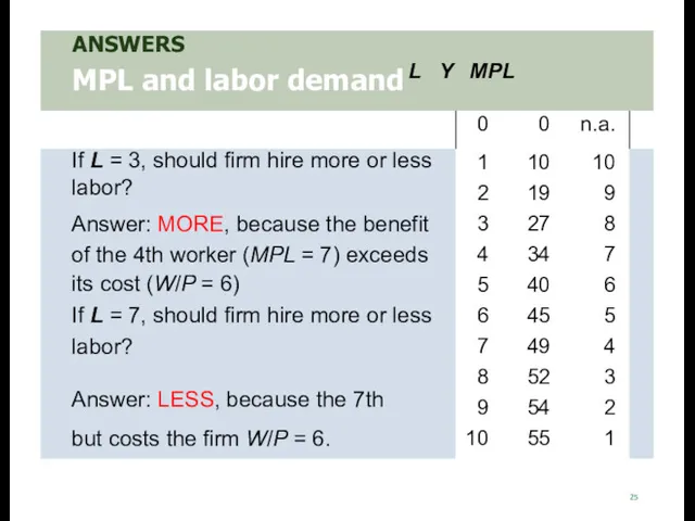
worker adds MPL = 4 units of output
25
worker adds MPL = 4 units of output
25
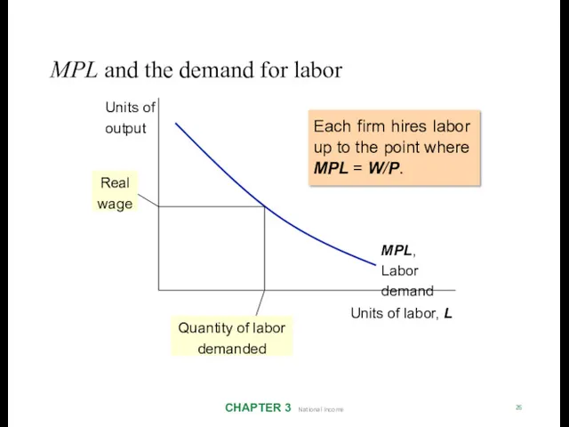
MPL and the demand for labor
CHAPTER 3 National Income
26
Each firm hires
MPL and the demand for labor
CHAPTER 3 National Income
26
Each firm hires
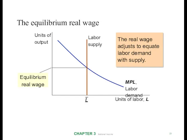
The equilibrium real wage
CHAPTER 3 National Income
27
The real wage adjusts to
The equilibrium real wage
CHAPTER 3 National Income
27
The real wage adjusts to
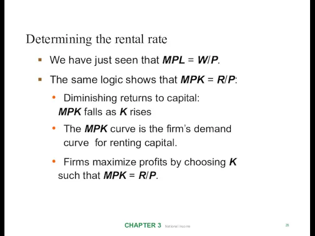
Determining the rental rate
CHAPTER 3 National Income
28
We have just seen that
Determining the rental rate
CHAPTER 3 National Income
28
We have just seen that
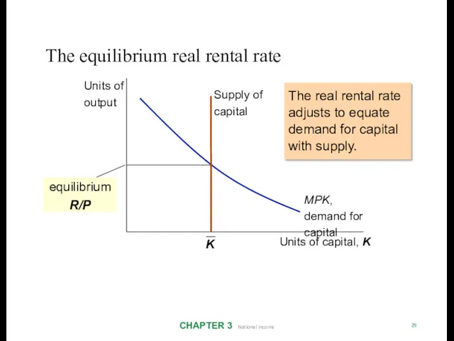
The equilibrium real rental rate
CHAPTER 3 National Income
29
The real rental rate
The equilibrium real rental rate
CHAPTER 3 National Income
29
The real rental rate

The neoclassical theory of distribution
CHAPTER 3 National Income
30
States that each factor
The neoclassical theory of distribution
CHAPTER 3 National Income
30
States that each factor
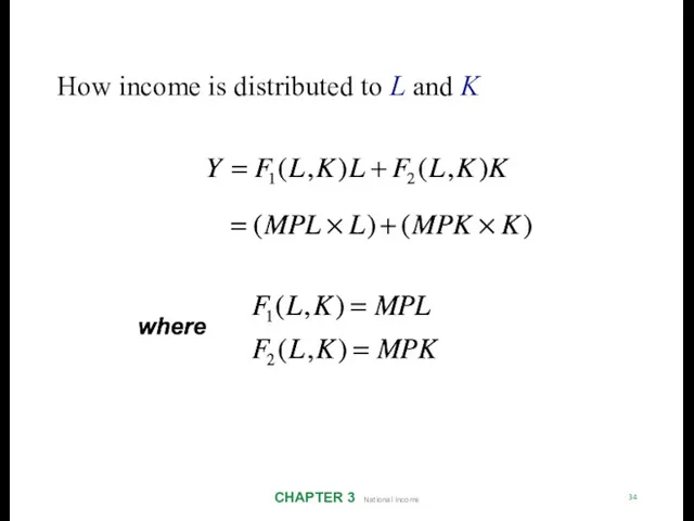
How income is distributed to L and K
CHAPTER 3 National Income
31
Total
How income is distributed to L and K
CHAPTER 3 National Income
31
Total
How income is distributed to L and K
CHAPTER 3 National Income
32
How income is distributed to L and K
CHAPTER 3 National Income
32
How income is distributed to L and K
CHAPTER 3 National Income
33
How income is distributed to L and K
CHAPTER 3 National Income
33
How income is distributed to L and K
CHAPTER 3 National Income
34
How income is distributed to L and K
CHAPTER 3 National Income
34
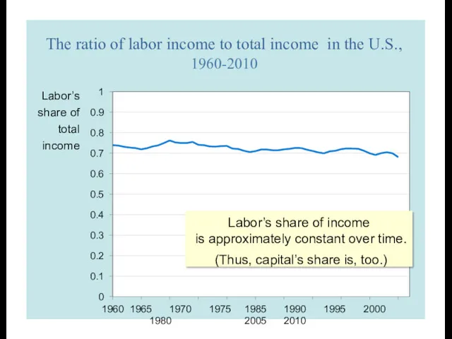
0.1
0
0.2
0.3
0.4
0.7
0.6
0.5
0.8
0.9
1
1960
1965 1970 1975 1980
1985 1990 1995 2000 2005 2010
The ratio of labor income to total income in the U.S.,
0.1
0
0.2
0.3
0.4
0.7
0.6
0.5
0.8
0.9
1
1960
1965 1970 1975 1980
1985 1990 1995 2000 2005 2010
The ratio of labor income to total income in the U.S.,
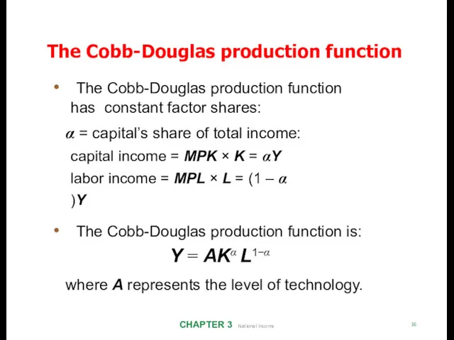
The Cobb-Douglas production function has constant factor shares:
CHAPTER 3 National
The Cobb-Douglas production function has constant factor shares:
CHAPTER 3 National
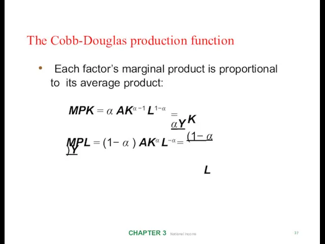
The Cobb-Douglas production function
CHAPTER 3 National Income
37
Each factor’s marginal product
The Cobb-Douglas production function
CHAPTER 3 National Income
37
Each factor’s marginal product
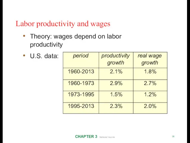
Labor productivity and wages
CHAPTER 3 National Income
38
Theory: wages depend on labor
Labor productivity and wages
CHAPTER 3 National Income
38
Theory: wages depend on labor
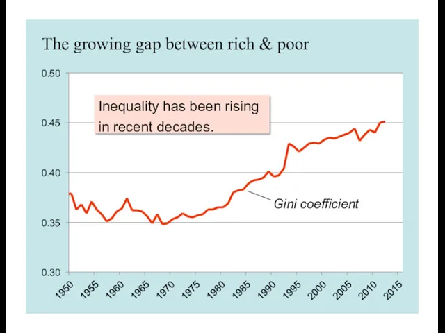
The growing gap between rich & poor
0.30
0.45
0.50
0.40
Gini coefficient
0.35
Inequality has been rising
The growing gap between rich & poor
0.30
0.45
0.50
0.40
Gini coefficient
0.35
Inequality has been rising

Explanations for rising inequality
CHAPTER 3 National Income
40
Rise in capital’s share of
Explanations for rising inequality
CHAPTER 3 National Income
40
Rise in capital’s share of

Outline of model
CHAPTER 3 National Income
41
A closed economy, market-clearing model
Supply side
DONE
Outline of model
CHAPTER 3 National Income
41
A closed economy, market-clearing model
Supply side
DONE
Demand for goods and services
CHAPTER 3 National Income
42
Components of aggregate demand:
C
Demand for goods and services
CHAPTER 3 National Income
42
Components of aggregate demand:
C
Consumption, C
CHAPTER 3 National Income
43
Disposable income is total income minus total
Consumption, C
CHAPTER 3 National Income
43
Disposable income is total income minus total
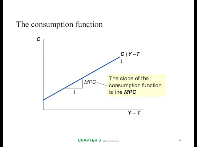
The consumption function
CHAPTER 3 National Income
44
C
Y – T
C (Y –T )
1
MPC
The
The consumption function
CHAPTER 3 National Income
44
C
Y – T
C (Y –T )
1
MPC
The
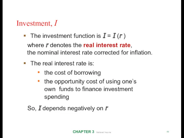
Investment, I
CHAPTER 3 National Income
45
The investment function is I = I
Investment, I
CHAPTER 3 National Income
45
The investment function is I = I
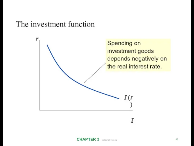
The investment function
CHAPTER 3 National Income
46
r
I (r )
I
Spending on investment goods
The investment function
CHAPTER 3 National Income
46
r
I (r )
I
Spending on investment goods

Government spending, G
CHAPTER 3 National Income
47
G = govt spending on goods
Government spending, G
CHAPTER 3 National Income
47
G = govt spending on goods
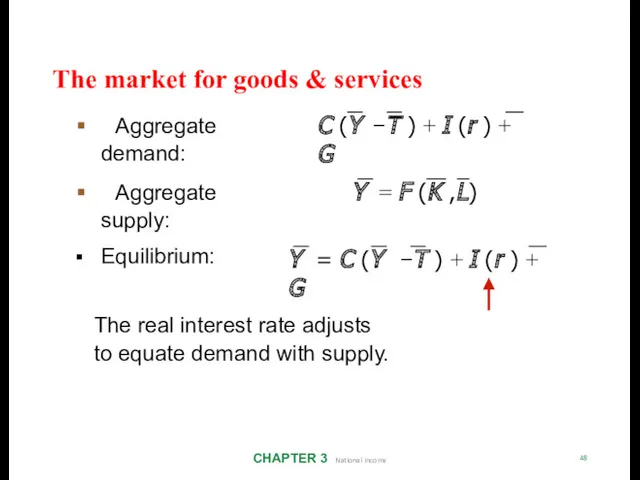
The market for goods & services
CHAPTER 3 National Income
48
Aggregate demand:
The market for goods & services
CHAPTER 3 National Income
48
Aggregate demand:
The loanable funds market
CHAPTER 3 National Income
49
A simple supply–demand model of
The loanable funds market
CHAPTER 3 National Income
49
A simple supply–demand model of
Demand for funds: investment
CHAPTER 3 National Income
50
The demand for loanable funds
Demand for funds: investment
CHAPTER 3 National Income
50
The demand for loanable funds
Loanable funds demand curve
CHAPTER 3 National Income
51
r
I (r )
I
The investment curve
Loanable funds demand curve
CHAPTER 3 National Income
51
r
I (r )
I
The investment curve
Supply of funds: saving
CHAPTER 3 National Income
52
The supply of loanable funds
Supply of funds: saving
CHAPTER 3 National Income
52
The supply of loanable funds

Types of saving
CHAPTER 3 National Income
53
Private saving Public saving
= (Y –
Types of saving
CHAPTER 3 National Income
53
Private saving Public saving
= (Y –
Notation: Δ = change in a variable
CHAPTER 3 National Income
54
For any variable
Notation: Δ = change in a variable
CHAPTER 3 National Income
54
For any variable
NOW YOU TRY
Calculate the change in saving
55
Suppose MPC = 0.8 and
NOW YOU TRY
Calculate the change in saving
55
Suppose MPC = 0.8 and
ANSWERS
Calculate the change in saving
56
ΔS = ΔY− ΔC−Δ G
= Δ Y − 0.8(Δ
ANSWERS
Calculate the change in saving
56
ΔS = ΔY− ΔC−Δ G
= Δ Y − 0.8(Δ

57
CHAPTER 3 National Income
Budget surpluses and deficits
If T > G,
57
CHAPTER 3 National Income
Budget surpluses and deficits
If T > G,
1940-2016
Percent of GDP
10
5
0
-5
-10
-15
-20
-25
-30
-35
1940
1950
1960
1970
1980
1990
2000
2010
U.S. federal government surplus/deficit
1940-2016
Percent of GDP
10
5
0
-5
-10
-15
-20
-25
-30
-35
1940
1950
1960
1970
1980
1990
2000
2010
U.S. federal government surplus/deficit
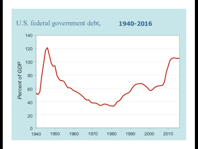
U.S. federal government debt,
1940-2016
Percent of GDP
140
120
100
80
60
40
20
0
1940
1950
1960
1970
1980
1990
2000
2010
U.S. federal government debt,
1940-2016
Percent of GDP
140
120
100
80
60
40
20
0
1940
1950
1960
1970
1980
1990
2000
2010
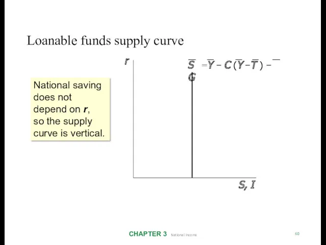
Loanable funds supply curve
CHAPTER 3 National Income
60
r
S, I
S =Y − C (Y −T )
Loanable funds supply curve
CHAPTER 3 National Income
60
r
S, I
S =Y − C (Y −T )
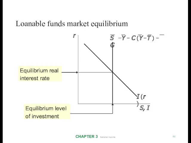
Loanable funds market equilibrium
CHAPTER 3 National Income
61
r
S, I
I (r )
S =Y − C
Loanable funds market equilibrium
CHAPTER 3 National Income
61
r
S, I
I (r )
S =Y − C
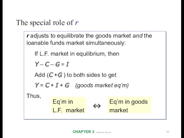
The special role of r
CHAPTER 3 National Income
62
r adjusts to equilibrate
The special role of r
CHAPTER 3 National Income
62
r adjusts to equilibrate
Digression: mastering models
CHAPTER 3 National Income
63
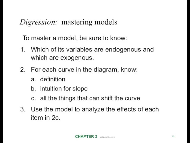
To master a model, be sure to
Digression: mastering models
CHAPTER 3 National Income
63
To master a model, be sure to
Mastering the loanable funds model
CHAPTER 3 National Income
64
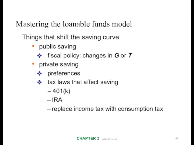
Things that shift the
Mastering the loanable funds model
CHAPTER 3 National Income
64
Things that shift the
CASE STUDY:
The Reagan Deficits
CHAPTER 3 National Income
65
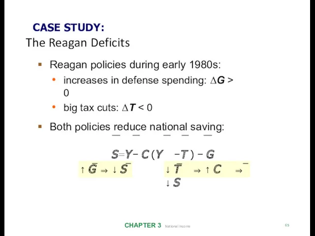
Reagan policies during early 1980s:
increases
CASE STUDY:
The Reagan Deficits
CHAPTER 3 National Income
65
Reagan policies during early 1980s:
increases
CASE STUDY:
The Reagan Deficits
CHAPTER 3 National Income
66
r
S, I
S 1
I (r )
r1
I1
r2
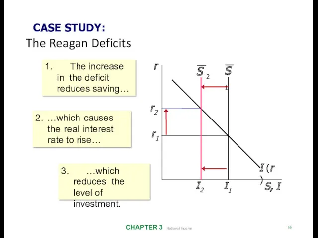
2.
CASE STUDY:
The Reagan Deficits
CHAPTER 3 National Income
66
r
S, I
S 1
I (r )
r1
I1
r2
2.
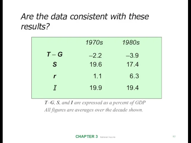
Are the data consistent with these results?
CHAPTER 3 National Income
67
T–G, S,
Are the data consistent with these results?
CHAPTER 3 National Income
67
T–G, S,
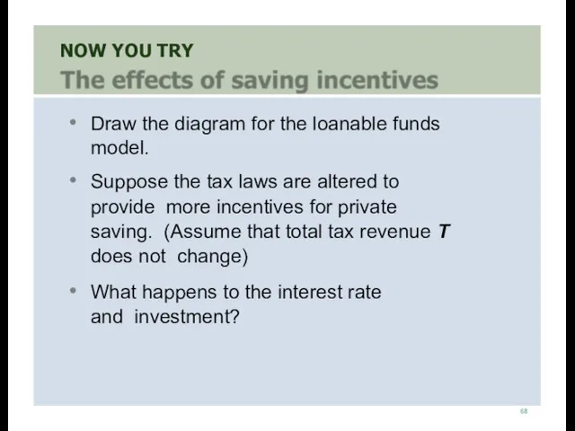
NOW YOU TRY
68
Draw the diagram for the loanable funds model.
Suppose the
NOW YOU TRY
68
Draw the diagram for the loanable funds model.
Suppose the
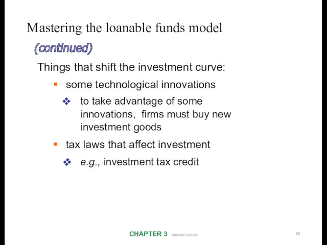
Mastering the loanable funds model
CHAPTER 3 National Income
69
(continued)
Things that shift the
Mastering the loanable funds model
CHAPTER 3 National Income
69
(continued)
Things that shift the
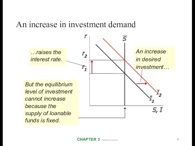
An increase in investment demand
CHAPTER 3 National Income
79
An increase in desired
An increase in investment demand
CHAPTER 3 National Income
79
An increase in desired
Saving and the interest rate
CHAPTER 3 National Income
71
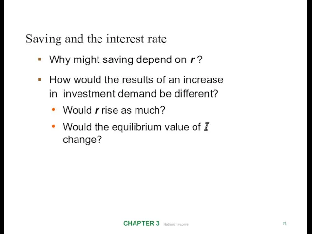
Why might saving depend
Saving and the interest rate
CHAPTER 3 National Income
71
Why might saving depend
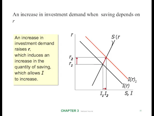
An increase in investment demand when saving depends on r
CHAPTER 3
An increase in investment demand when saving depends on r
CHAPTER 3
C H A P T E R S U M M A
C H A P T E R S U M M A
C H A P T E R S U M M A
C H A P T E R S U M M A
 Формализация задач мониторинга и оценки новаций в проектировании регионального устойчивого инновационного развития
 Международное разделение труда в мировом хозяйстве
 Типы экономических систем
 Платежный баланс
 Цена. Основные функции цены
 Економічний аналіз та методи економічної оцінки в сфері охорони здоров’я
 Искусство и экономика. Художественный аукцион
 Итоги производственной и финансово-экономической деятельности эксплуатационного локомотивного депо Уссурийск
 Особенности методики школьного экономического образования. (Лекция 2)
 Аралас экономика және қазіргі қоғамдық өндіріс қызмет етуінің объективті нысаны
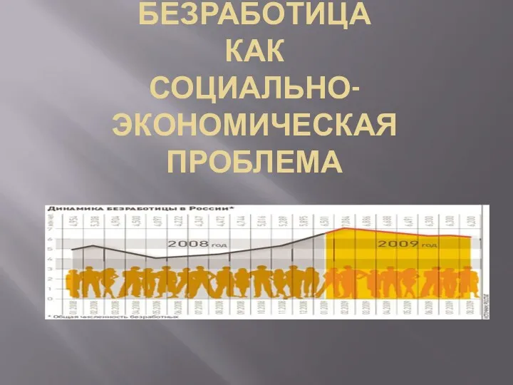 Безработица как социально-экономическая проблема
 Общая характеристика рыночной экономики
 Анализ экономических показателей на основе применения метода динамических рядов
 Организация труда и трудовые отношения
 Экономическая свобода и социальная ответственность
 Prezentatsia_kursovoy_raboty
 Финансы как экономическая категория
 Экономика. Экономические блага и ресурсы
 Forecast combinations
 Definition capacity
 Правовые и экономические особенности закупки ТРУ отдельными юридическими лицами
 Мектеп кеме-білім теңіз
 Народосбережение. Демографическая ситуация, основные причины сложившегося положения дел, задачи народосбережения
 Сельское хозяйство Великобритании
 Система национальных счетов. Основные макроэкономические показатели
 Собственность, как экономическая категория
 Планирование материально-технического обеспечения и механизации. Планирование труда и прибыли
 Современная система ценообразования в энергетике. Оптовый рынок электроэнергии (мощности)