- Rotordynamics

Содержание
- 2. Inventory Number: 002764 1st Edition ANSYS Release: 12.0 Published Date: April 30, 2009 Registered Trademarks: ANSYS®
- 3. Agenda Why / what is Rotordynamics Equations for rotating structures Rotating and stationary reference frame Elements
- 4. High speed machinery such as Turbine Engine Rotors, Computer Disk Drives, etc. Very small rotor-stator clearances
- 5. Rotordynamics features Pre-processing: Appropriate element formulation for all geometries Gyroscopic moments generated by rotating parts Bearings
- 6. Rotordynamics features Post-processing Campbell diagrams Mode animation Orbit plots Transient plots and animations User’s guide Advanced
- 7. Rotordynamics - theory
- 8. Rotordynamics - theory In a stationary reference frame, we are solving the following equation: M, C
- 9. Coriolis matrix in dynamic analyses: Rotordynamics - theory Dynamic equation in rotating reference frame
- 10. Rotordynamics – theory
- 11. Rotordynamics - theory
- 12. Rotordynamics - theory Acceleration of point mass due to deflection Po – P (small displacement -
- 13. Rotordynamics - reference frames Rotordynamics simulation can be performed in two different reference frames: Stationary reference
- 14. Our focus in this presentation Rotordynamics - reference frames
- 15. Applicable ANSYS element types Rotordynamics - ANSYS elements
- 16. Rotating damping Considered if the rotating structure has: structural damping (MP, DAMP or BETAD) or a
- 17. General axisymmetric element In v12.0, the new SOLID272 (4nodes) and SOLID273 (8nodes) generalized axisymmetric elements: are
- 18. Generalized axisymmetric element Allow a very fast setup of axisymmetric 3D parts: Slice an axisymmetric 3D
- 19. Bearing coefficients may be function of rotational speed: Typical Rotor – Bearing System Bearings
- 20. Bearings 2D spring/damper with cross-coupling terms: Real constants are stiffness and damping coefficients and can vary
- 21. Rotordynamics - commands Coriolis / Gyroscopic effect CORIOLIS, Option, --, --, RefFrame, RotDamp Applies the Coriolis
- 22. Rotordynamics - commands
- 23. OMEGA, OMEGX, OMEGY, OMEGZ, KSPIN Rotational velocity of the structure. SOLUTION: inertia CMOMEGA, CM_NAME, OMEGAX, OMEGAY,
- 24. RSTMAC, file1, Lstep1, Sbstep1, file2, Lstep2, Sbstep2, TolerN, MacLim, Cname, KeyPrint Filei First Jobname (DB and
- 25. Rotordynamics - Campbell diagram Variation of the rotor natural frequency with respect to rotor speed ω
- 26. Rotordynamics - Campbell diagram Campbell diagram PLCAMP, Option, SLOPE, UNIT, FREQB, Cname, STABVAL Option Flag to
- 27. Rotordynamics – multi-spool rotors More than 1 spool and / or non-rotating parts, use components (CM)
- 28. Rotordynamics – multi-spool rotor Whirl animation (ANHARM command)
- 29. Campbell diagrams & whirl Variation of the rotor natural frequencies with respect to rotor speed ω
- 30. Rotor whirl Forward whirl: when ω and the whirl motion are rotating in the same direction
- 31. Orbit plots In a plane perpendicular to the spin axis, the orbit of a node is
- 32. Rotordynamics – forced response Possible excitations caused by rotation velocity ω are: Unbalance (ω) Coupling misalignment
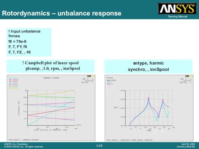
- 33. SYNCHRO, ratio, cname ratio The ratio between the frequency of excitation, f, and the frequency of
- 34. ! Example of input file /prep7 … F0=m*r F, node, fy, F0 F, node, fz, ,
- 35. ! Campbell plot of inner spool plcamp, ,1.0, rpm, , innSpool ! Input unbalance forces f0
- 36. Stability Self-excited vibrations in a rotating structure cause an increase of the vibration amplitude over time
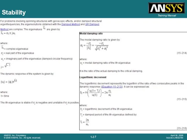
- 37. Stability
- 38. Stability Stable at 30,000 rpm (3141.6 rad/sec) Unstable at 60,000 rpm (6283.2 rad/sec)
- 39. Rotordynamics analysis guide New at release 12.0 Provides a detailed description of capabilities Provides guidelines for
- 40. Sample models available
- 41. Some examples
- 42. Validation examples
- 43. Generic validation model Modal analysis of a 3D beam (solid elements), ω=30000 rpm Excellent agreement between
- 44. Nelson rotor (beams & bearings)
- 45. Instability analysis – transient analysis 30,000 rpm; closed trajectory: stable 60,000 rpm; open trajectory: unstable Rotor
- 46. Instability analysis – modal analysis All complex frequencies’ real parts are negative: stable One complex frequency
- 47. Effect of rotating damping
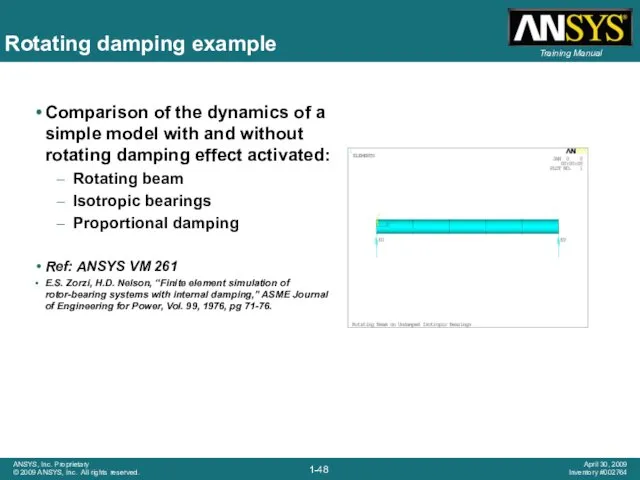
- 48. Rotating damping example Comparison of the dynamics of a simple model with and without rotating damping
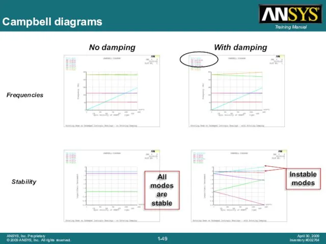
- 49. Campbell diagrams Frequencies Stability
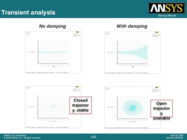
- 50. Transient analysis No damping With damping Closed trajectory, stable Open trajectory, unstable
- 51. Rotordynamics with ANSYS Workbench
- 52. Geometry & model definition The database contains a generic steel rotor created in ANSYS DesignModeler to
- 53. Bearing definition The standard Simulation springs are changed to bearing elements utilizing the parameter, _sid to
- 54. Solution settings for modal analysis A commands object inserted into the analysis branch switches the default
- 55. Solution information While the solution is running, the solution output can be monitored. The output shown
- 56. Modal results Complex modal results are shown in the tabular view of the results. Complex eigenshapes
- 57. Animated modal shape
- 58. Compressor model Solid model & casing simulation
- 59. Compressor: free-free testing apparatus used for initial model calibration +Z Courtesy of Trane, a business of
- 60. Compressor: location of lumped representation of impellers and bearings Courtesy of Trane, a business of American
- 61. Compressor: SOLID185 mesh of shaft Very stiff symmetric contact between axial segments
- 62. Compressor: forward whirl mode Courtesy of Trane, a business of American Standard, Inc.
- 63. Compressor: backward whirl mode Courtesy of Trane, a business of American Standard, Inc.
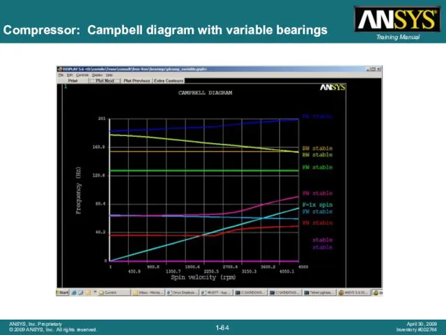
- 64. Compressor: Campbell diagram with variable bearings
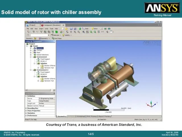
- 65. Solid model of rotor with chiller assembly Courtesy of Trane, a business of American Standard, Inc.
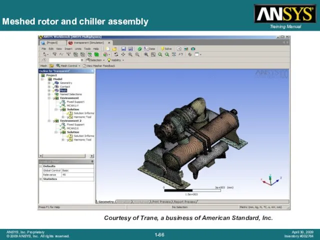
- 66. Meshed rotor and chiller assembly Courtesy of Trane, a business of American Standard, Inc.
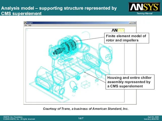
- 67. Analysis model – supporting structure represented by CMS superelement Courtesy of Trane, a business of American
- 68. Analysis model Courtesy of Trane, a business of American Standard, Inc.
- 69. Typical mode animation Courtesy of Trane, a business of American Standard, Inc.
- 70. Blower shaft model Transient startup & effect of prestress
- 71. Blower shaft - model Impeller to pump hot hydrogen rich mix of gas and liquid into
- 72. Blower shaft - modal analysis Frequencies and corresponding mode shapes orbits
- 73. Blower shaft – modal analysis Frequencies Stability
- 74. Blower shaft – critical speed
- 75. Blower shaft – unbalance response Harmonic response to disk unbalance - Disk eccentricity is .002” -
- 76. Blower Shaft – unbalance response Bearings reactions Forward bearing is more loaded than rear one as
- 77. Blower shaft – start up Transient analysis Ramped rotational velocity over 4 seconds Unbalance transient forces
- 78. Blower shaft – start up Displacement UY and UZ at disk zoom on critical speed passage
- 79. Blower shaft – start up Transient orbits 0 to 4 seconds 3 to 4 seconds As
- 80. Blower shaft – prestress Include prestress due to thermal loading: Thermal body load up to 1500
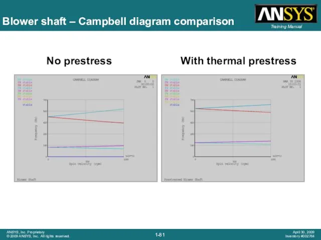
- 81. Blower shaft – Campbell diagram comparison No prestress With thermal prestress
- 82. Demo’s Agenda 3D model Point mass by user Automatic Rigid Body B.C. / Remote displacement Bearing
- 83. Rotordynamics with ANSYS Workbench A workflow example
- 84. Storyboard The geometry is provided in form of a Parasolid file Part of the shaft must
- 85. Project view Upper part of the schematics defines the simulation process (geometry to mesh to simulation)
- 86. Geometry setup Geometry is imported in Design Modeler A part of the shaft is redesigned with
- 87. Geometry details Part of the original shaft is removed and recreated with parametric radius 3D Model
- 88. Mesh The model is meshed using the WB meshing tools
- 89. Simulation Simulation is performed using an APDL script that defines: Element types Bearings Boundary conditions Solutions
- 90. APDL script Spring1 component comes from named selection Mesh transferred as mesh200 elements, converted to solid272
- 91. Simulation results The APDL scripts can create plots and animations The results can also be analyzed
- 92. Mode animation (expanded view)
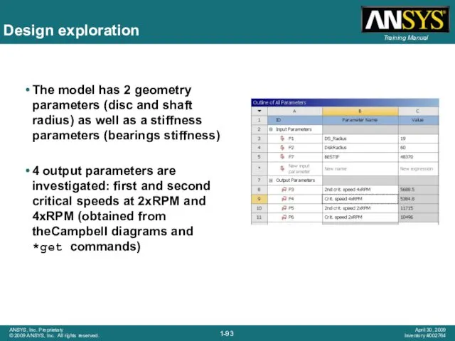
- 93. Design exploration The model has 2 geometry parameters (disc and shaft radius) as well as a
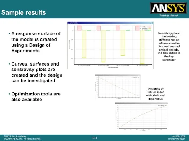
- 94. Sample results A response surface of the model is created using a Design of Experiments Curves,
- 96. Скачать презентацию
Inventory Number: 002764
1st Edition
ANSYS Release: 12.0
Published Date: April 30, 2009
Registered Trademarks:
ANSYS®
Inventory Number: 002764
1st Edition
ANSYS Release: 12.0
Published Date: April 30, 2009
Registered Trademarks:
ANSYS®
Agenda
Why / what is Rotordynamics
Equations for rotating structures
Rotating and stationary reference
Agenda
Why / what is Rotordynamics
Equations for rotating structures
Rotating and stationary reference
High speed machinery such as Turbine Engine Rotors, Computer Disk Drives,
High speed machinery such as Turbine Engine Rotors, Computer Disk Drives,
Rotordynamics features
Pre-processing:
Appropriate element formulation for all geometries
Gyroscopic moments generated by rotating
Rotordynamics features
Pre-processing:
Appropriate element formulation for all geometries
Gyroscopic moments generated by rotating
Rotordynamics features
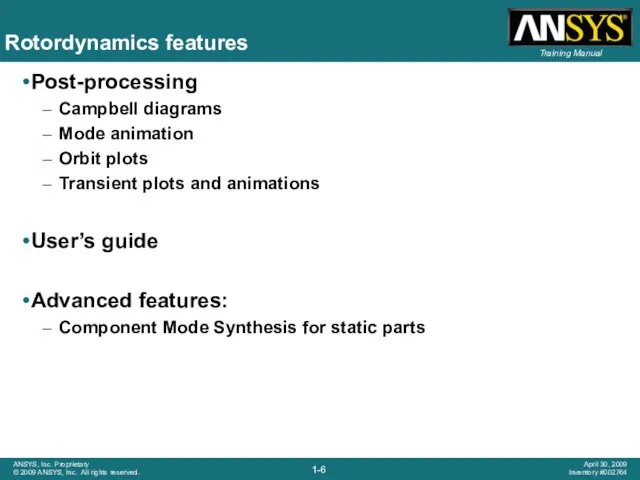
Post-processing
Campbell diagrams
Mode animation
Orbit plots
Transient plots and animations
User’s guide
Advanced features:
Component Mode
Rotordynamics features
Post-processing
Campbell diagrams
Mode animation
Orbit plots
Transient plots and animations
User’s guide
Advanced features:
Component Mode
Rotordynamics - theory
Rotordynamics - theory
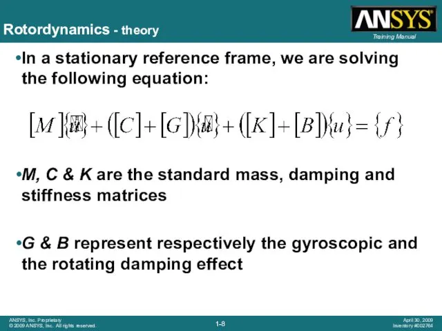
Rotordynamics - theory
In a stationary reference frame, we are solving the
Rotordynamics - theory
In a stationary reference frame, we are solving the
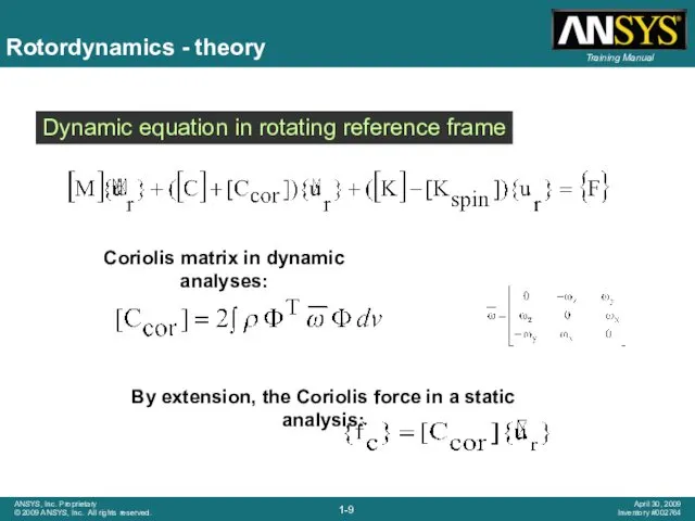
Coriolis matrix in dynamic analyses:
Rotordynamics - theory
Dynamic equation in rotating reference
Coriolis matrix in dynamic analyses:
Rotordynamics - theory
Dynamic equation in rotating reference
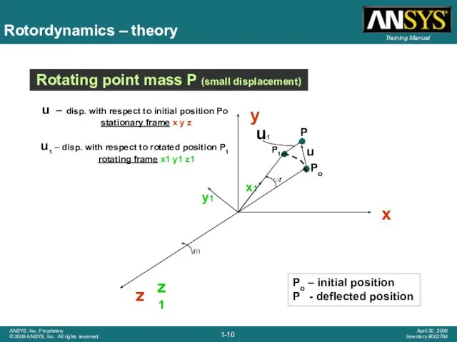
Rotordynamics – theory
Rotordynamics – theory
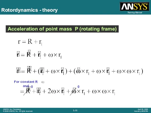
Rotordynamics - theory
Rotordynamics - theory
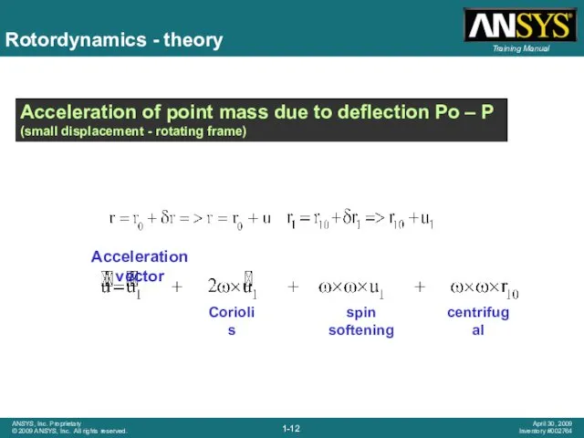
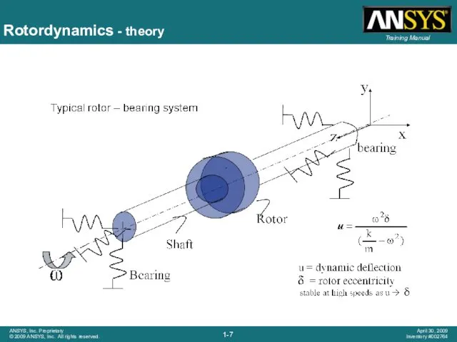
Rotordynamics - theory
Acceleration of point mass due to deflection Po –
Rotordynamics - theory
Acceleration of point mass due to deflection Po –
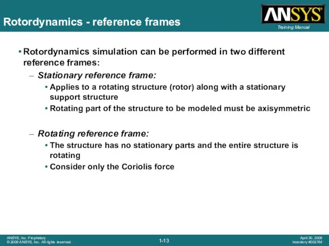
Rotordynamics - reference frames
Rotordynamics simulation can be performed in two different
Rotordynamics - reference frames
Rotordynamics simulation can be performed in two different
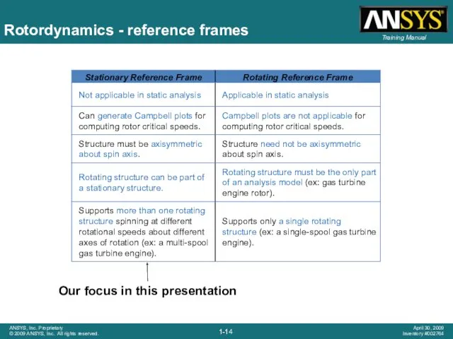
Our focus in this presentation
Rotordynamics - reference frames
Our focus in this presentation
Rotordynamics - reference frames
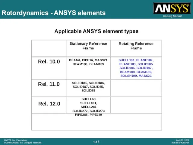
Applicable ANSYS element types
Rotordynamics - ANSYS elements
Applicable ANSYS element types
Rotordynamics - ANSYS elements
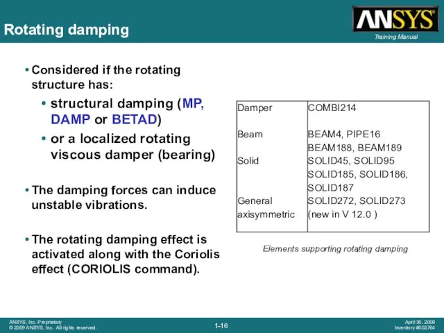
Rotating damping
Considered if the rotating structure has:
structural damping (MP, DAMP or
Rotating damping
Considered if the rotating structure has:
structural damping (MP, DAMP or
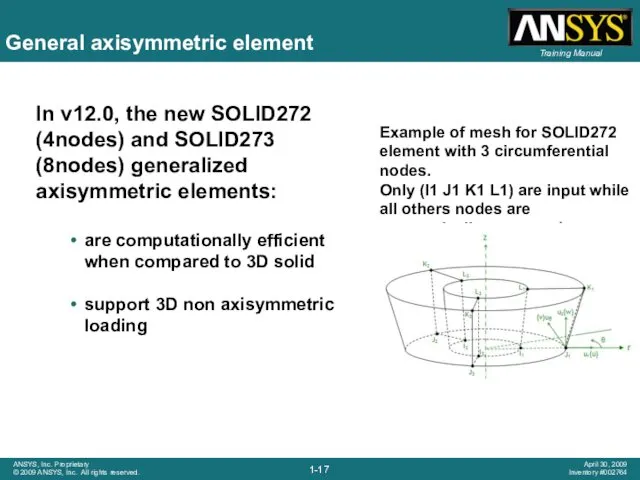
General axisymmetric element
In v12.0, the new SOLID272 (4nodes) and SOLID273 (8nodes)
General axisymmetric element
In v12.0, the new SOLID272 (4nodes) and SOLID273 (8nodes)
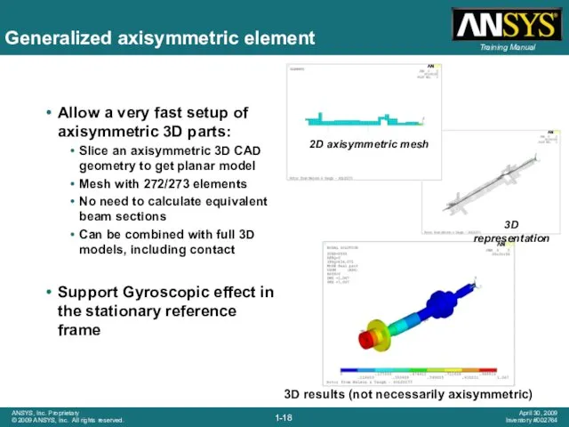
Generalized axisymmetric element
Allow a very fast setup of axisymmetric 3D parts:
Slice
Generalized axisymmetric element
Allow a very fast setup of axisymmetric 3D parts:
Slice
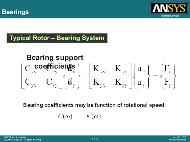
Bearing coefficients may be function of rotational speed:
Typical Rotor – Bearing
Bearing coefficients may be function of rotational speed:
Typical Rotor – Bearing
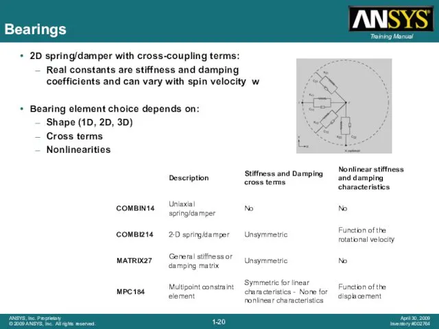
Bearings
2D spring/damper with cross-coupling terms:
Real constants are stiffness and damping
Bearings
2D spring/damper with cross-coupling terms:
Real constants are stiffness and damping
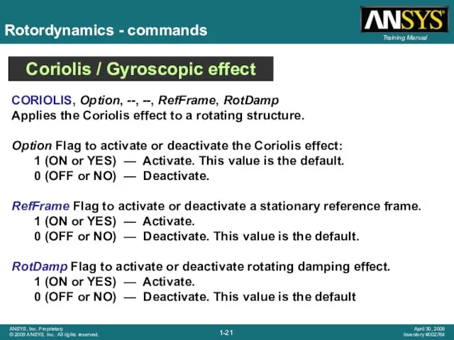
Rotordynamics - commands
Coriolis / Gyroscopic effect
CORIOLIS, Option, --, --, RefFrame, RotDamp
Applies
Rotordynamics - commands
Coriolis / Gyroscopic effect
CORIOLIS, Option, --, --, RefFrame, RotDamp Applies
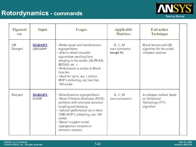
Rotordynamics - commands
Rotordynamics - commands
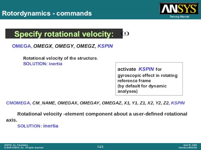
OMEGA, OMEGX, OMEGY, OMEGZ, KSPIN
Rotational velocity of the structure.
SOLUTION:
OMEGA, OMEGX, OMEGY, OMEGZ, KSPIN
Rotational velocity of the structure.
SOLUTION:
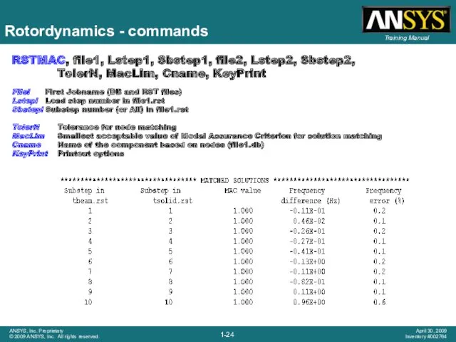
RSTMAC, file1, Lstep1, Sbstep1, file2, Lstep2, Sbstep2,
TolerN, MacLim, Cname, KeyPrint
Filei
RSTMAC, file1, Lstep1, Sbstep1, file2, Lstep2, Sbstep2,
TolerN, MacLim, Cname, KeyPrint
Filei
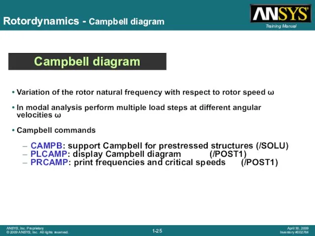
Rotordynamics - Campbell diagram
Variation of the rotor natural frequency with respect
Rotordynamics - Campbell diagram
Variation of the rotor natural frequency with respect
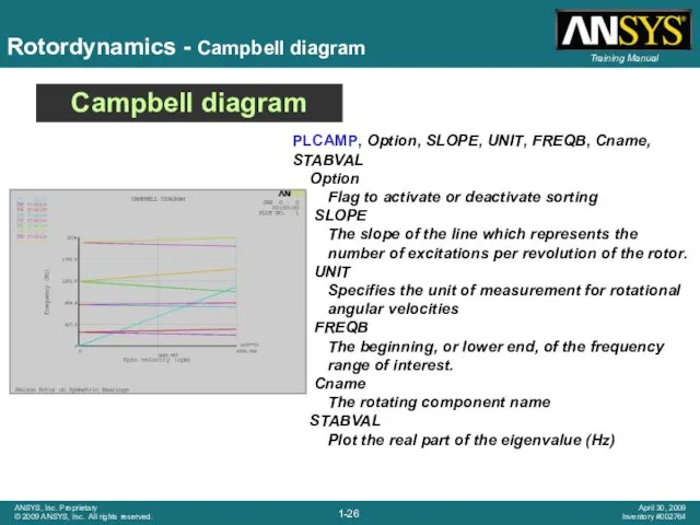
Rotordynamics - Campbell diagram
Campbell diagram
PLCAMP, Option, SLOPE, UNIT, FREQB, Cname, STABVAL
Rotordynamics - Campbell diagram
Campbell diagram
PLCAMP, Option, SLOPE, UNIT, FREQB, Cname, STABVAL
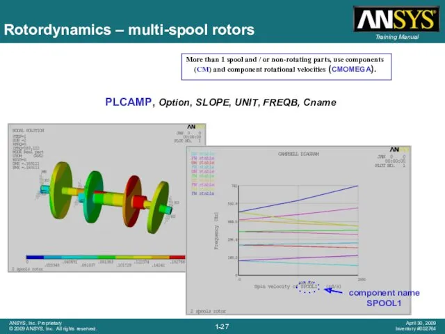
Rotordynamics – multi-spool rotors
More than 1 spool and / or non-rotating
Rotordynamics – multi-spool rotors
More than 1 spool and / or non-rotating
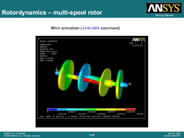
Rotordynamics – multi-spool rotor
Whirl animation (ANHARM command)
Rotordynamics – multi-spool rotor
Whirl animation (ANHARM command)
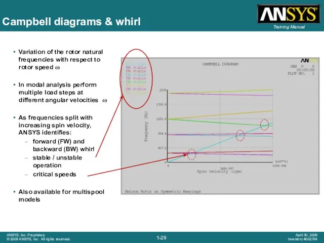
Campbell diagrams & whirl
Variation of the rotor natural frequencies with respect
Campbell diagrams & whirl
Variation of the rotor natural frequencies with respect
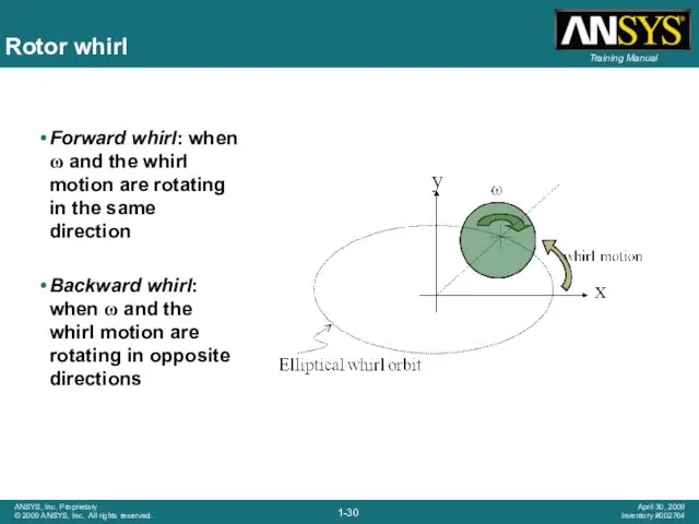
Rotor whirl
Forward whirl: when ω and the whirl motion are rotating
Rotor whirl
Forward whirl: when ω and the whirl motion are rotating
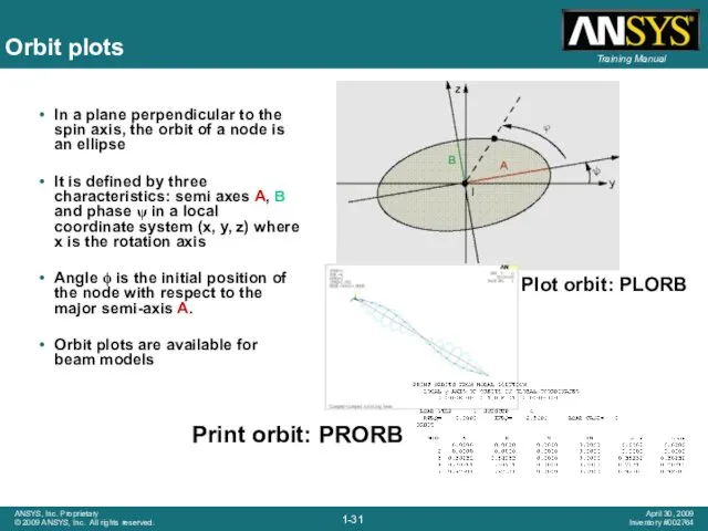
Orbit plots
In a plane perpendicular to the spin axis, the orbit
Orbit plots
In a plane perpendicular to the spin axis, the orbit
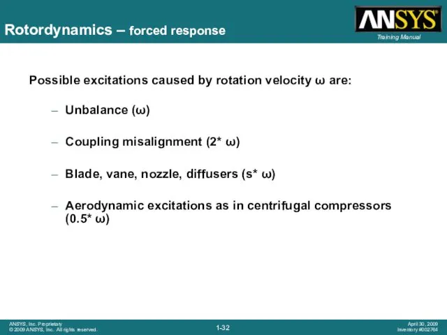
Rotordynamics – forced response
Possible excitations caused by rotation velocity ω are:
Unbalance
Rotordynamics – forced response
Possible excitations caused by rotation velocity ω are:
Unbalance
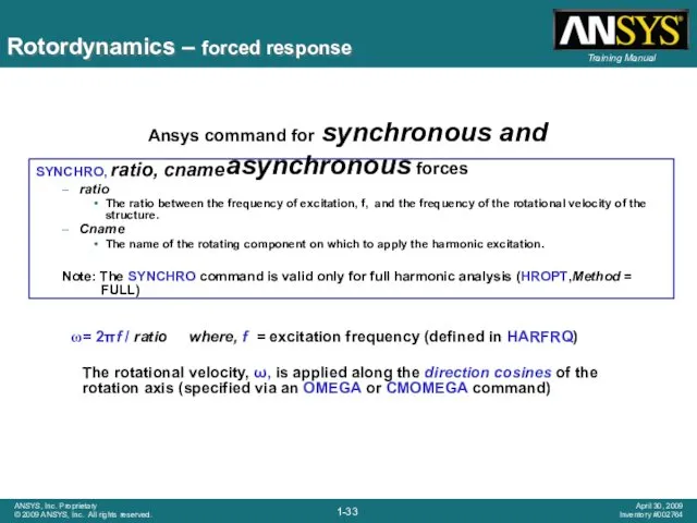
SYNCHRO, ratio, cname
ratio
The ratio between the frequency of excitation, f, and
SYNCHRO, ratio, cname
ratio
The ratio between the frequency of excitation, f, and
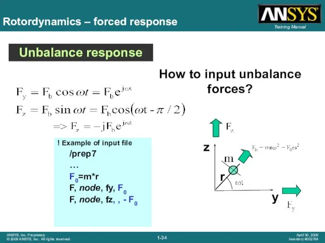
! Example of input file
/prep7
…
F0=m*r
F, node, fy, F0
F, node, fz,
! Example of input file
/prep7
…
F0=m*r
F, node, fy, F0
F, node, fz,
! Campbell plot of inner spool
plcamp, ,1.0, rpm, , innSpool
!
! Campbell plot of inner spool
plcamp, ,1.0, rpm, , innSpool
!
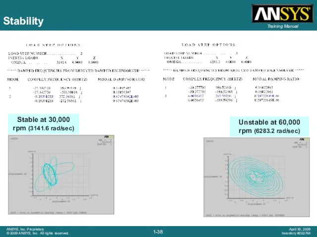
Stability
Self-excited vibrations in a rotating structure cause an increase of the
Stability
Self-excited vibrations in a rotating structure cause an increase of the
Stability
Stability
Stability
Stable at 30,000 rpm (3141.6 rad/sec)
Unstable at 60,000 rpm (6283.2 rad/sec)
Stability
Stable at 30,000 rpm (3141.6 rad/sec)
Unstable at 60,000 rpm (6283.2 rad/sec)
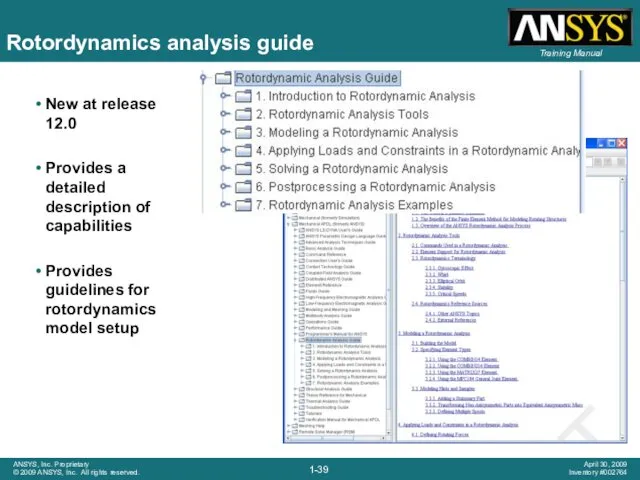
Rotordynamics analysis guide
New at release 12.0
Provides a detailed description of
Rotordynamics analysis guide
New at release 12.0
Provides a detailed description of
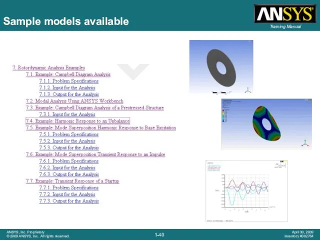
Sample models available
Sample models available

Some examples
Some examples

Validation examples
Validation examples
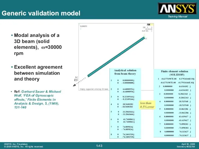
Generic validation model
Modal analysis of a 3D beam (solid elements), ω=30000
Generic validation model
Modal analysis of a 3D beam (solid elements), ω=30000
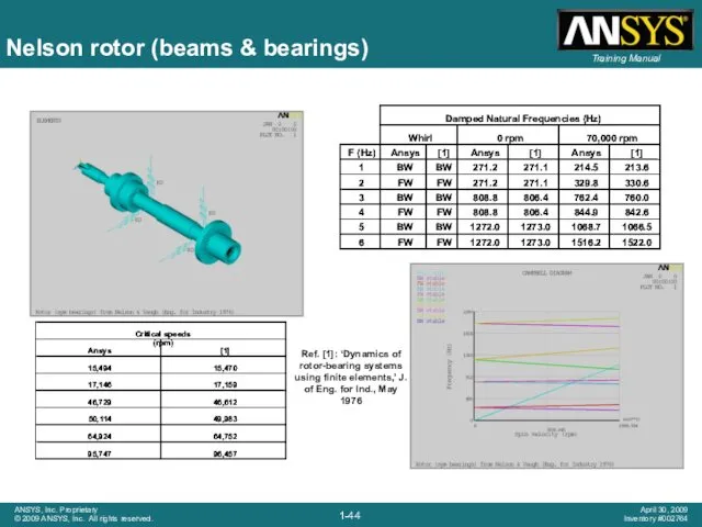
Nelson rotor (beams & bearings)
Nelson rotor (beams & bearings)
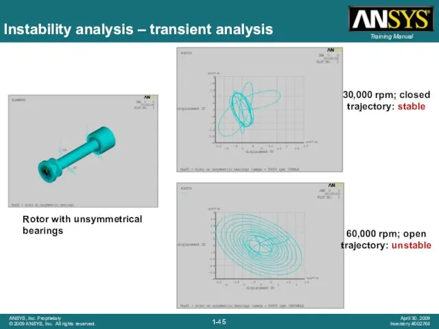
Instability analysis – transient analysis
30,000 rpm; closed trajectory: stable
60,000 rpm; open
Instability analysis – transient analysis
30,000 rpm; closed trajectory: stable
60,000 rpm; open
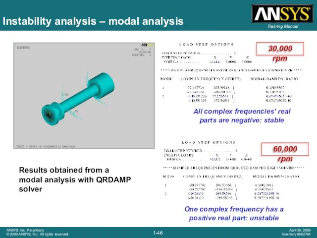
Instability analysis – modal analysis
All complex frequencies’ real parts are negative:
Instability analysis – modal analysis
All complex frequencies’ real parts are negative:
Effect of rotating damping
Effect of rotating damping
Rotating damping example
Comparison of the dynamics of a simple model with
Rotating damping example
Comparison of the dynamics of a simple model with
Campbell diagrams
Frequencies
Stability
Campbell diagrams
Frequencies
Stability
Transient analysis
No damping
With damping
Closed trajectory, stable
Open trajectory, unstable
Transient analysis
No damping
With damping
Closed trajectory, stable
Open trajectory, unstable
Rotordynamics with ANSYS Workbench
Rotordynamics with ANSYS Workbench
Geometry & model definition
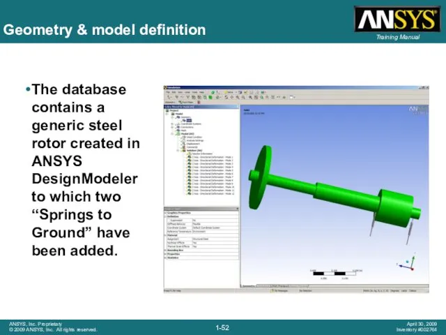
The database contains a generic steel rotor created
Geometry & model definition
The database contains a generic steel rotor created
Bearing definition
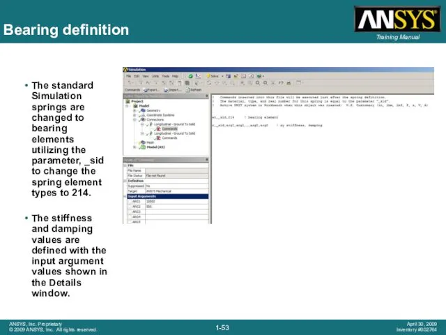
The standard Simulation springs are changed to bearing elements utilizing
Bearing definition
The standard Simulation springs are changed to bearing elements utilizing
Solution settings for modal analysis
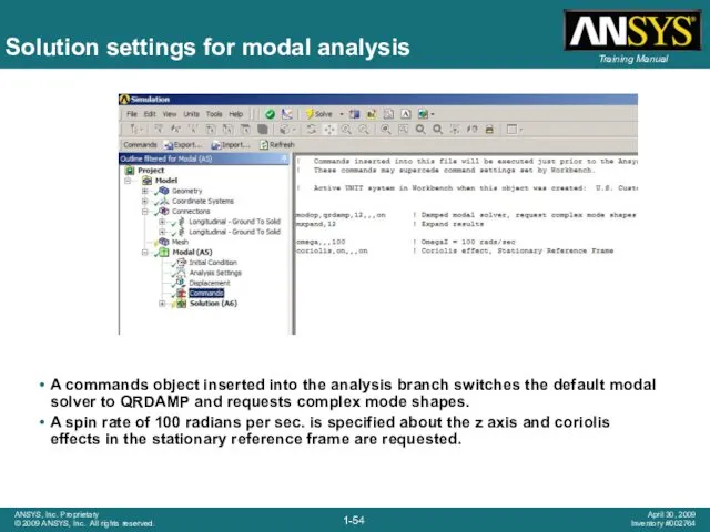
A commands object inserted into the
Solution settings for modal analysis
A commands object inserted into the
Solution information
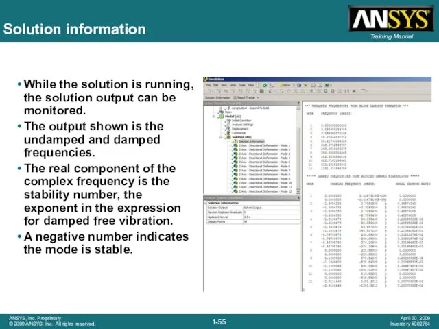
While the solution is running, the solution output can be
Solution information
While the solution is running, the solution output can be
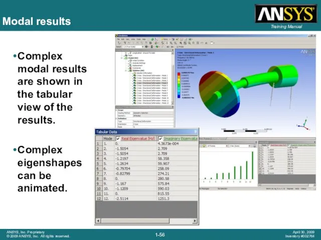
Modal results
Complex modal results are shown in the tabular view of
Modal results
Complex modal results are shown in the tabular view of
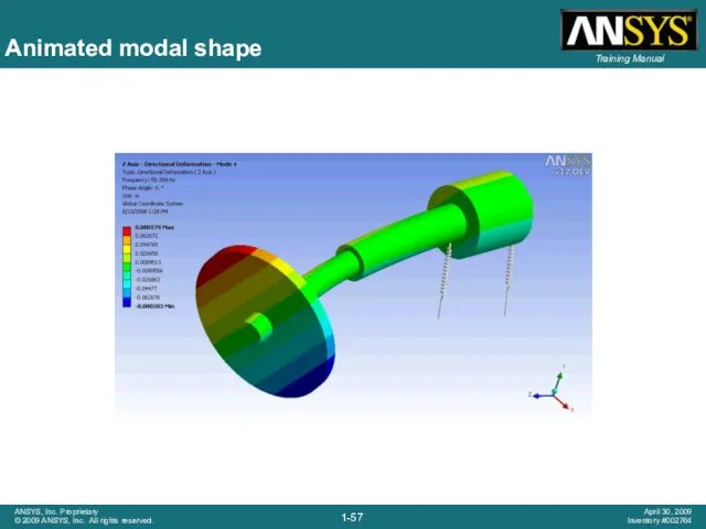
Animated modal shape
Animated modal shape
Compressor model
Solid model & casing simulation
Compressor model
Solid model & casing simulation
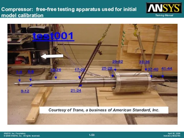
Compressor: free-free testing apparatus used for initial model calibration
+Z
Courtesy of Trane,
Compressor: free-free testing apparatus used for initial model calibration
+Z
Courtesy of Trane,
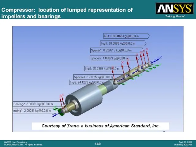
Compressor: location of lumped representation of impellers and bearings
Courtesy of Trane,
Compressor: location of lumped representation of impellers and bearings
Courtesy of Trane,
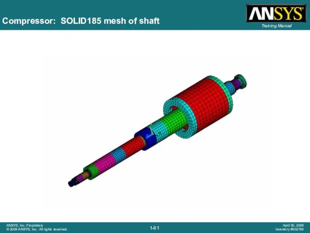
Compressor: SOLID185 mesh of shaft
Very stiff symmetric contact between axial segments
Compressor: SOLID185 mesh of shaft
Very stiff symmetric contact between axial segments
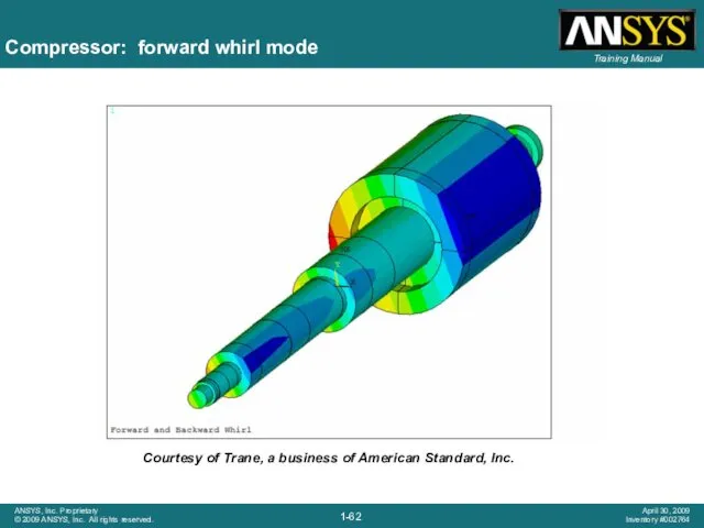
Compressor: forward whirl mode
Courtesy of Trane, a business of American Standard,
Compressor: forward whirl mode
Courtesy of Trane, a business of American Standard,
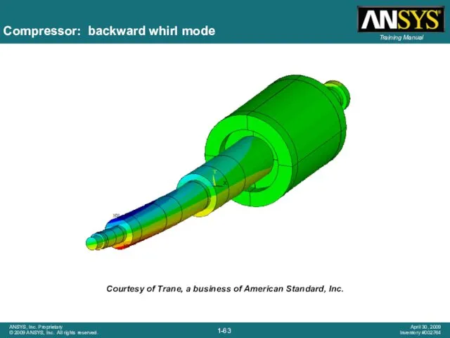
Compressor: backward whirl mode
Courtesy of Trane, a business of American Standard,
Compressor: backward whirl mode
Courtesy of Trane, a business of American Standard,
Compressor: Campbell diagram with variable bearings
Compressor: Campbell diagram with variable bearings
Solid model of rotor with chiller assembly
Courtesy of Trane, a business
Solid model of rotor with chiller assembly
Courtesy of Trane, a business
Meshed rotor and chiller assembly
Courtesy of Trane, a business of American
Meshed rotor and chiller assembly
Courtesy of Trane, a business of American
Analysis model – supporting structure represented by CMS superelement
Courtesy of Trane,
Analysis model – supporting structure represented by CMS superelement
Courtesy of Trane,
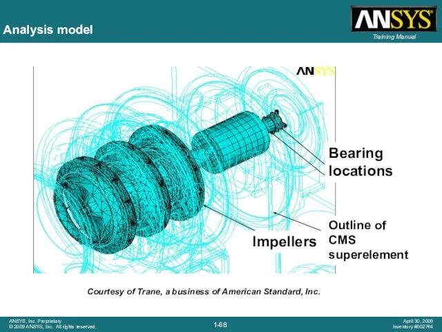
Analysis model
Courtesy of Trane, a business of American Standard, Inc.
Analysis model
Courtesy of Trane, a business of American Standard, Inc.
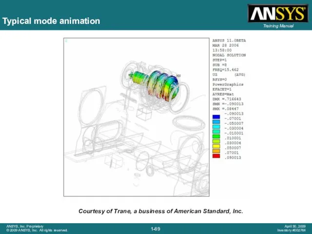
Typical mode animation
Courtesy of Trane, a business of American Standard, Inc.
Typical mode animation
Courtesy of Trane, a business of American Standard, Inc.

Blower shaft model
Transient startup & effect of prestress
Blower shaft model
Transient startup & effect of prestress
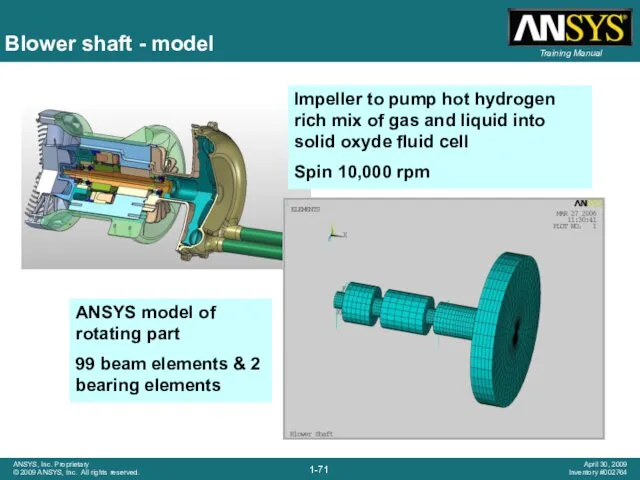
Blower shaft - model
Impeller to pump hot hydrogen rich mix of
Blower shaft - model
Impeller to pump hot hydrogen rich mix of
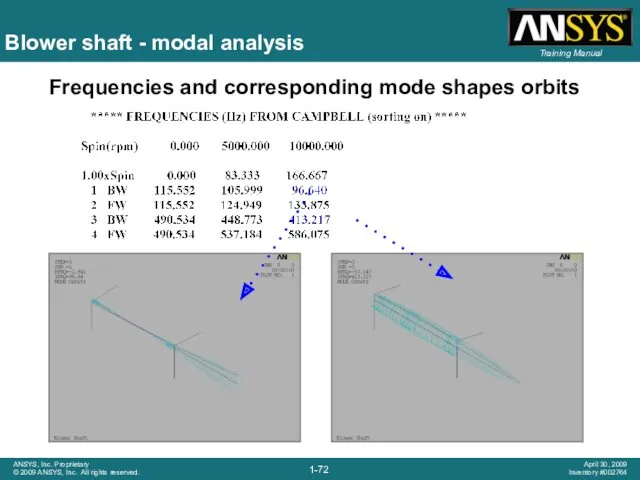
Blower shaft - modal analysis
Frequencies and corresponding mode shapes orbits
Blower shaft - modal analysis
Frequencies and corresponding mode shapes orbits
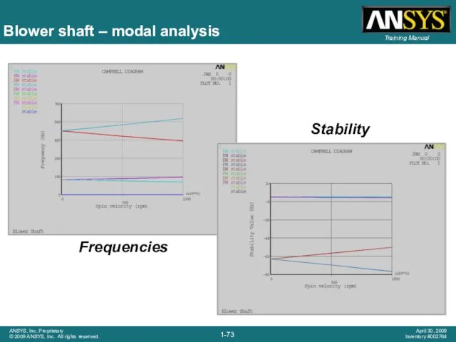
Blower shaft – modal analysis
Frequencies
Stability
Blower shaft – modal analysis
Frequencies
Stability
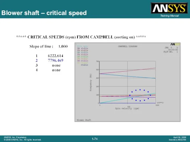
Blower shaft – critical speed
Blower shaft – critical speed
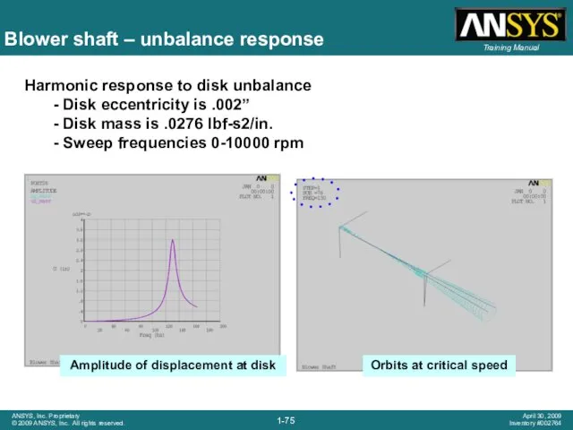
Blower shaft – unbalance response
Harmonic response to disk unbalance
- Disk eccentricity
Blower shaft – unbalance response
Harmonic response to disk unbalance
- Disk eccentricity
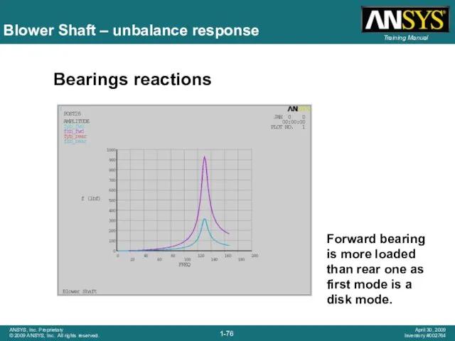
Blower Shaft – unbalance response
Bearings reactions
Forward bearing is more loaded than
Blower Shaft – unbalance response
Bearings reactions
Forward bearing is more loaded than
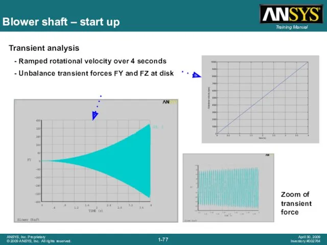
Blower shaft – start up
Transient analysis
Ramped rotational velocity over 4 seconds
Unbalance
Blower shaft – start up
Transient analysis
Ramped rotational velocity over 4 seconds
Unbalance
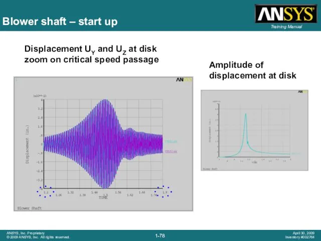
Blower shaft – start up
Displacement UY and UZ at disk zoom
Blower shaft – start up
Displacement UY and UZ at disk zoom
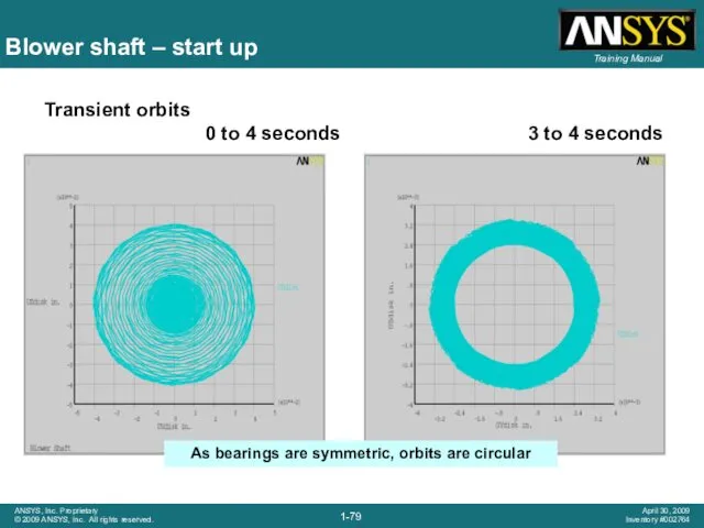
Blower shaft – start up
Transient orbits
0 to 4 seconds
3 to 4
Blower shaft – start up
Transient orbits
0 to 4 seconds
3 to 4
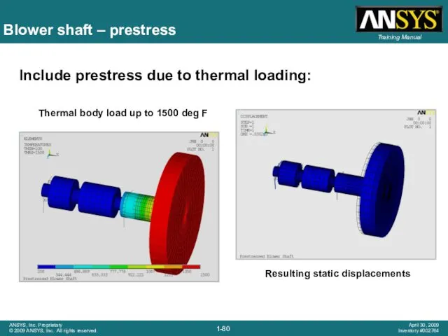
Blower shaft – prestress
Include prestress due to thermal loading:
Thermal body load
Blower shaft – prestress
Include prestress due to thermal loading:
Thermal body load
Blower shaft – Campbell diagram comparison
No prestress
With thermal prestress
Blower shaft – Campbell diagram comparison
No prestress
With thermal prestress
Demo’s Agenda
3D model
Point mass by user
Automatic Rigid Body
B.C. / Remote displacement
Bearing
Demo’s Agenda
3D model
Point mass by user
Automatic Rigid Body
B.C. / Remote displacement
Bearing
Rotordynamics with ANSYS Workbench
A workflow example
Rotordynamics with ANSYS Workbench
A workflow example
Storyboard
The geometry is provided in form of a Parasolid file
Part of
Storyboard
The geometry is provided in form of a Parasolid file
Part of
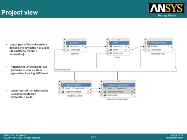
Project view
Upper part of the schematics defines the simulation process (geometry
Project view
Upper part of the schematics defines the simulation process (geometry
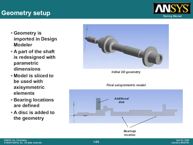
Geometry setup
Geometry is imported in Design Modeler
A part of the
Geometry setup
Geometry is imported in Design Modeler
A part of the
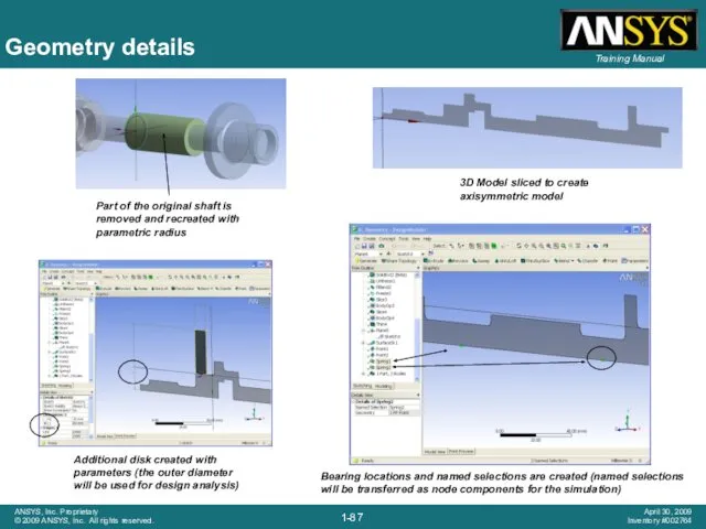
Geometry details
Part of the original shaft is removed and recreated with
Geometry details
Part of the original shaft is removed and recreated with
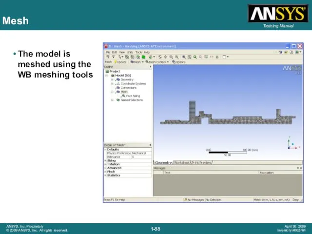
Mesh
The model is meshed using the WB meshing tools
Mesh
The model is meshed using the WB meshing tools
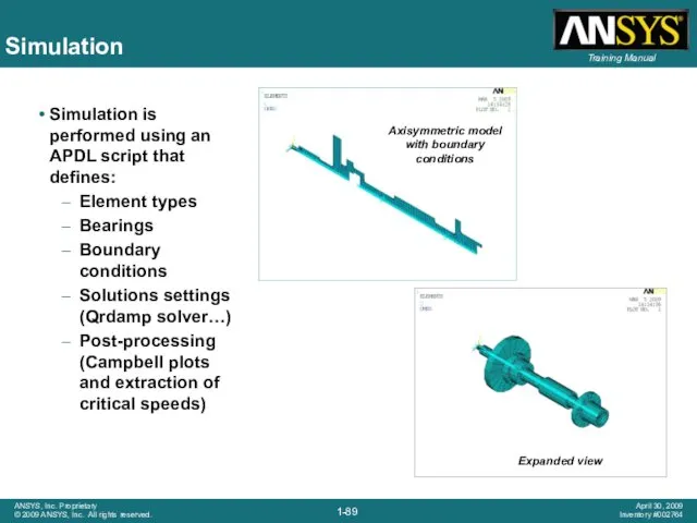
Simulation
Simulation is performed using an APDL script that defines:
Element types
Bearings
Boundary conditions
Solutions
Simulation
Simulation is performed using an APDL script that defines:
Element types
Bearings
Boundary conditions
Solutions
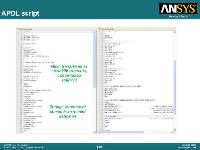
APDL script
Spring1 component comes from named selection
Mesh transferred as mesh200 elements,
APDL script
Spring1 component comes from named selection
Mesh transferred as mesh200 elements,
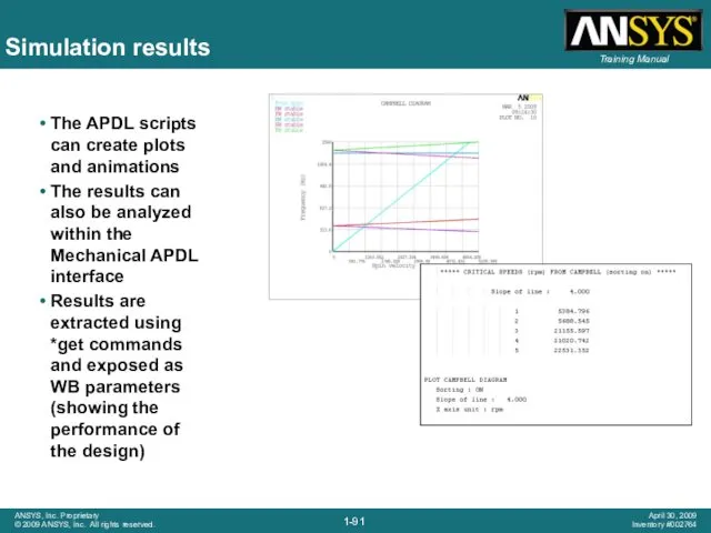
Simulation results
The APDL scripts can create plots and animations
The results can
Simulation results
The APDL scripts can create plots and animations
The results can
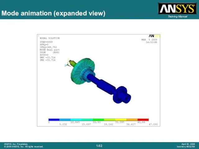
Mode animation (expanded view)
Mode animation (expanded view)
Design exploration
The model has 2 geometry parameters (disc and shaft radius)
Design exploration
The model has 2 geometry parameters (disc and shaft radius)
Sample results
A response surface of the model is created using a
Sample results
A response surface of the model is created using a
 Теплові насоси та кондиціонери
 Дисперсия света
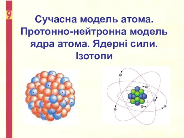 Сучасна модель атома. Протонно-нейтронна модель ядра атома. Ядерні сили. Ізотопи
 Физика. Эволюция взгляда на физическую картину мира
 конструктор урока по теме Постоянный ток
 Резание металла и проволоки слесарной ножовкой
 Отражение в горизонтальном зеркале
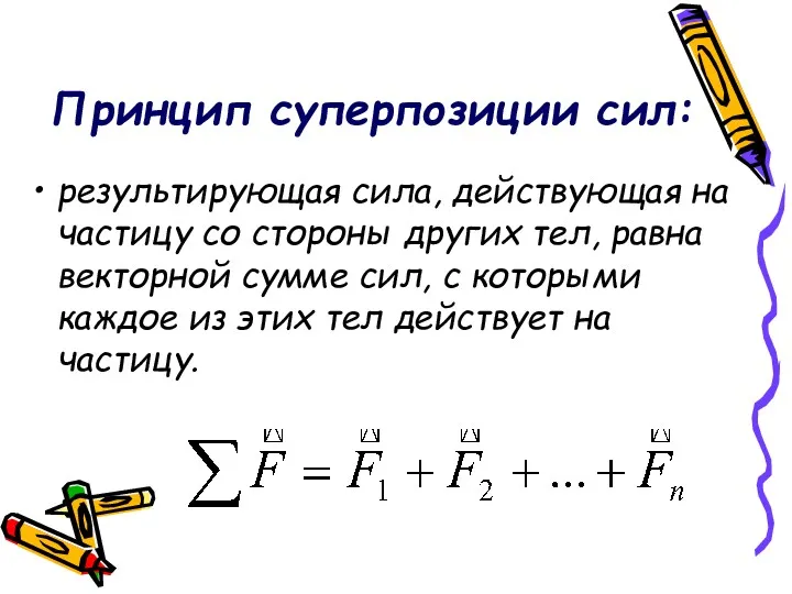 Принцип суперпозиции сил
 Плотность вещества. 7 класс
 Sm-Nd метод
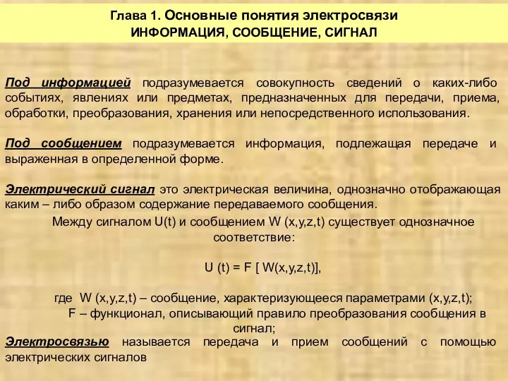 Основные понятия электросвязи. Информация, сообщение, сигнал
 Свободные колебания простых одномерных осцилляторов
 Електричний струм у різних середовищах
 Шкала электромагнитного излучения
 Кремний. Строение полупроводников
 Yüzey ve kompozi̇syon (9)
 Интерактивный урок Эксплуатация и ремонт. Возможные неисправности топливораздаточных колонок и способы их устранения
 Реактивное движение
 Изготовление столярного соединения УС-1
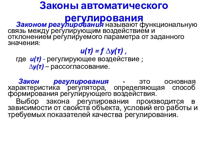 Законы автоматического регулирования
 Конспект урока по физике в 10 классе на тему Температура
 Испарение. Насыщенный и ненасыщенный пар
 Вертолет Ми-8МТВ. Несущий винт
 Chassis
 Emission spectrum of H
 Спектрофотометрия и спектрофлуориметрия
 Поляризация света. Лекция №3
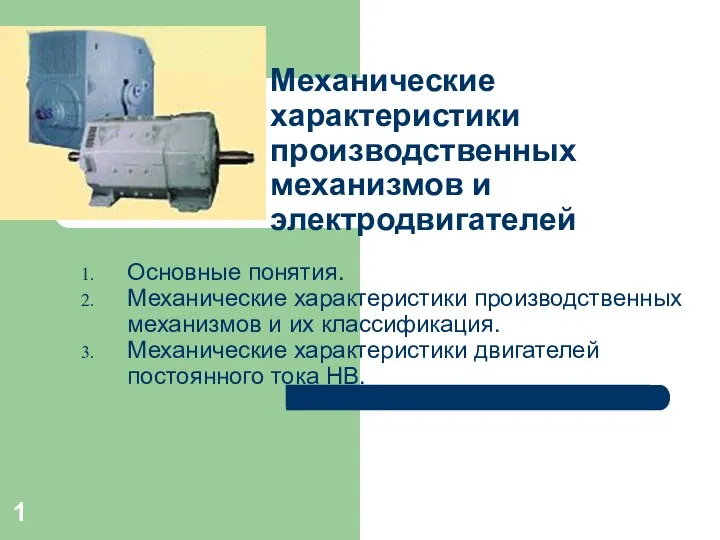 Механические характеристики производственных механизмов и электродвигателей