- 3D Viewing Pipeline

Содержание
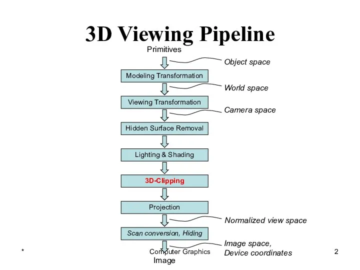
- 2. * Computer Graphics Normalized view space Modeling Transformation Viewing Transformation Lighting & Shading 3D-Clipping Projection Scan
- 3. Contents Introduction Clipping Volume Clipping Strategies Clipping Algorithm
- 4. * Computer Graphics 3D Clipping Just like the case in two dimensions, clipping removes objects that
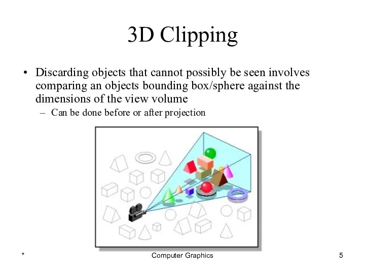
- 5. * Computer Graphics 3D Clipping Discarding objects that cannot possibly be seen involves comparing an objects
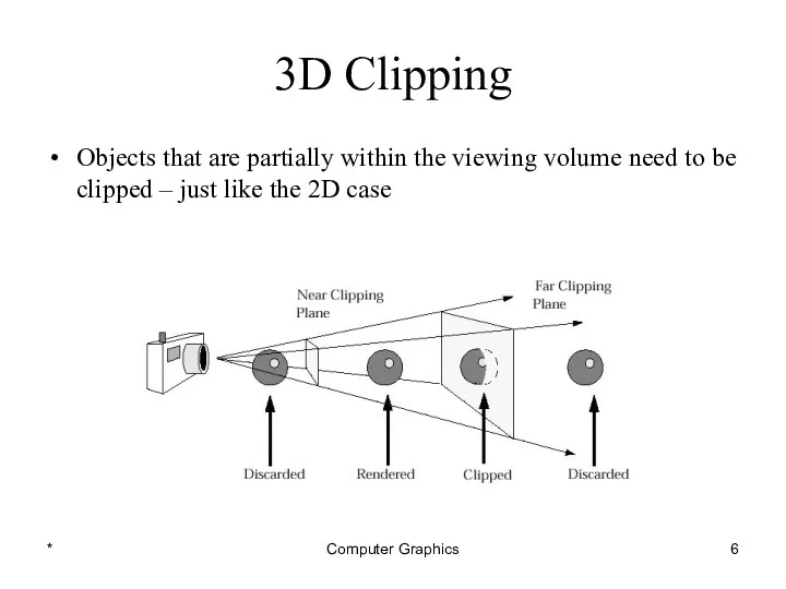
- 6. * Computer Graphics 3D Clipping Objects that are partially within the viewing volume need to be
- 7. Contents Introduction Clipping Volume Clipping Strategies Clipping Algorithm
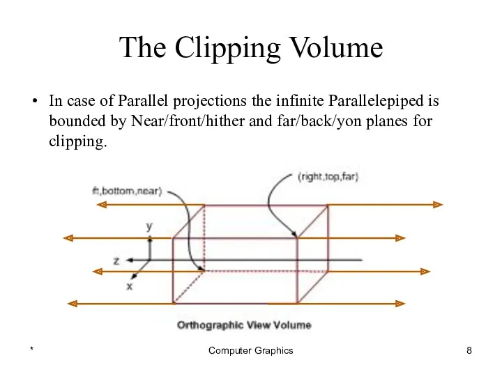
- 8. * Computer Graphics The Clipping Volume In case of Parallel projections the infinite Parallelepiped is bounded
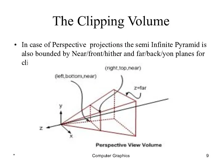
- 9. * Computer Graphics The Clipping Volume In case of Perspective projections the semi Infinite Pyramid is
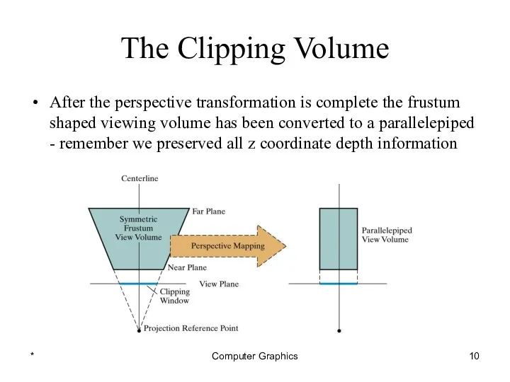
- 10. * Computer Graphics The Clipping Volume After the perspective transformation is complete the frustum shaped viewing
- 11. Contents Introduction Clipping Volume Clipping Strategies Clipping Algorithm
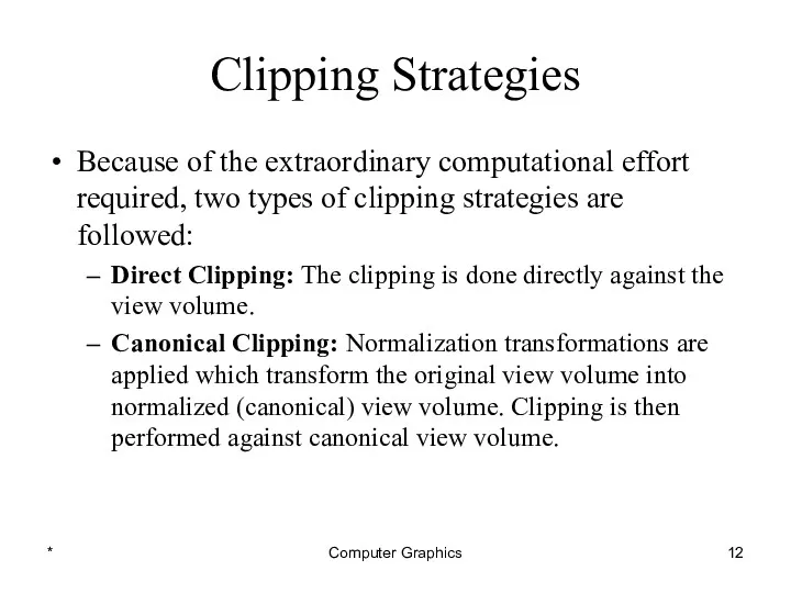
- 12. * Computer Graphics Clipping Strategies Because of the extraordinary computational effort required, two types of clipping
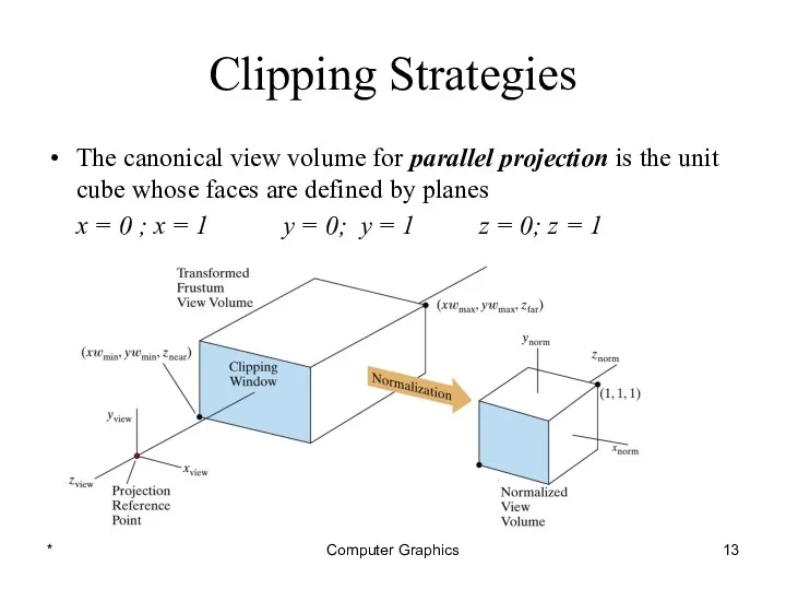
- 13. * Computer Graphics Clipping Strategies The canonical view volume for parallel projection is the unit cube
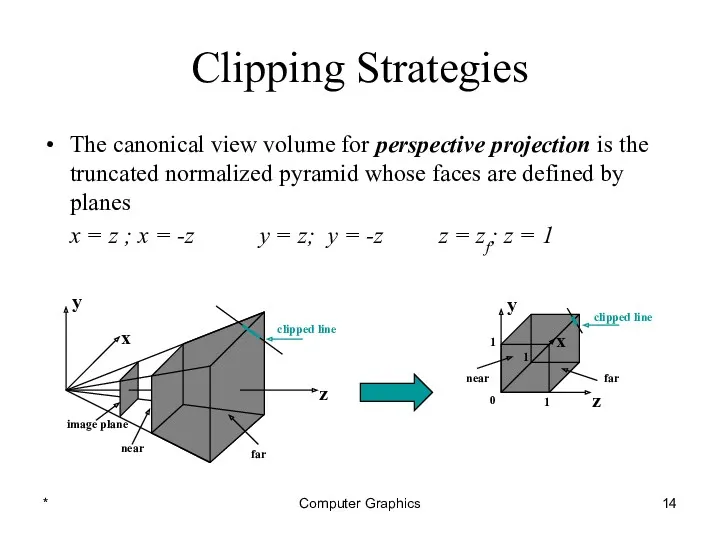
- 14. * Computer Graphics Clipping Strategies The canonical view volume for perspective projection is the truncated normalized
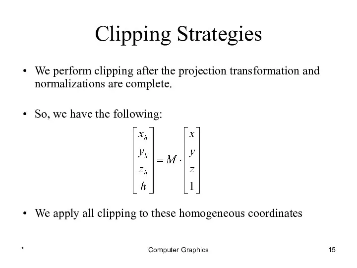
- 15. * Computer Graphics Clipping Strategies We perform clipping after the projection transformation and normalizations are complete.
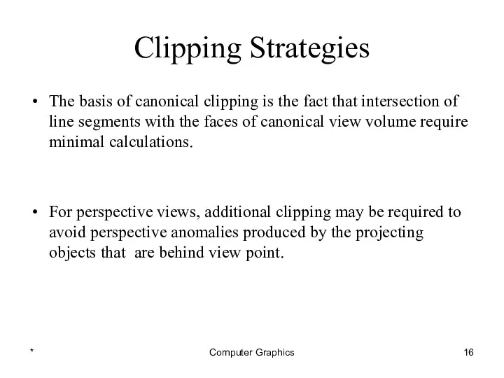
- 16. * Computer Graphics Clipping Strategies The basis of canonical clipping is the fact that intersection of
- 17. Contents Introduction Clipping Volume Clipping Strategies Clipping Algorithm
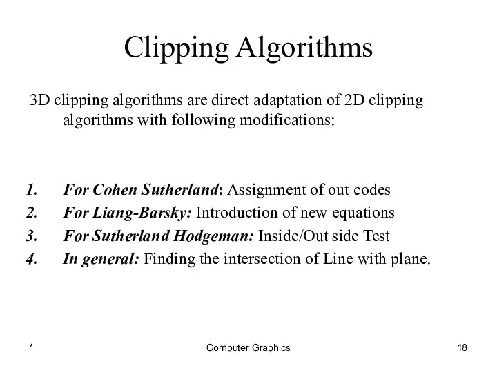
- 18. * Computer Graphics Clipping Algorithms 3D clipping algorithms are direct adaptation of 2D clipping algorithms with
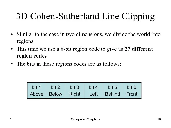
- 19. * Computer Graphics 3D Cohen-Sutherland Line Clipping Similar to the case in two dimensions, we divide
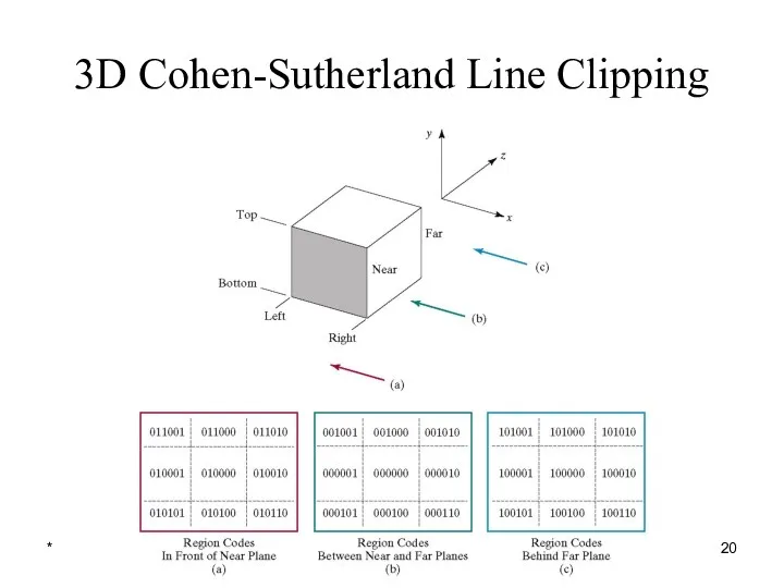
- 20. * Computer Graphics 3D Cohen-Sutherland Line Clipping
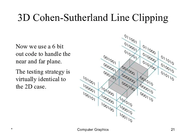
- 21. * Computer Graphics 3D Cohen-Sutherland Line Clipping Now we use a 6 bit out code to
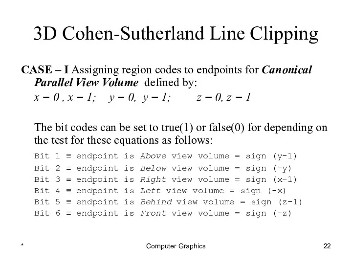
- 22. * Computer Graphics 3D Cohen-Sutherland Line Clipping CASE – I Assigning region codes to endpoints for
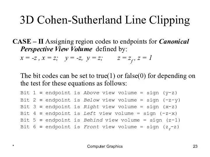
- 23. * Computer Graphics 3D Cohen-Sutherland Line Clipping CASE – II Assigning region codes to endpoints for
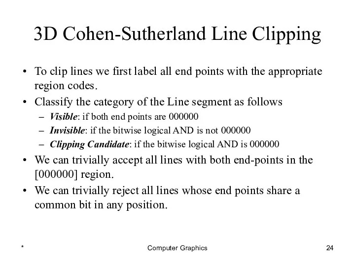
- 24. * Computer Graphics 3D Cohen-Sutherland Line Clipping To clip lines we first label all end points
- 25. * Computer Graphics 3D Cohen-Sutherland Line Clipping
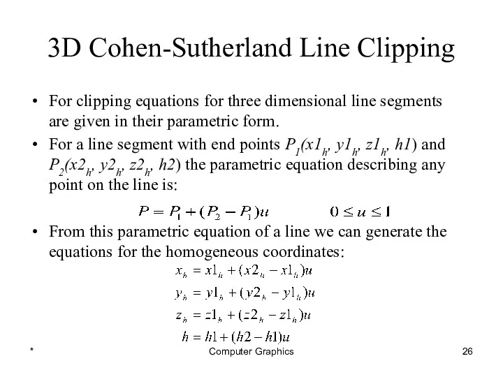
- 26. * Computer Graphics 3D Cohen-Sutherland Line Clipping For clipping equations for three dimensional line segments are
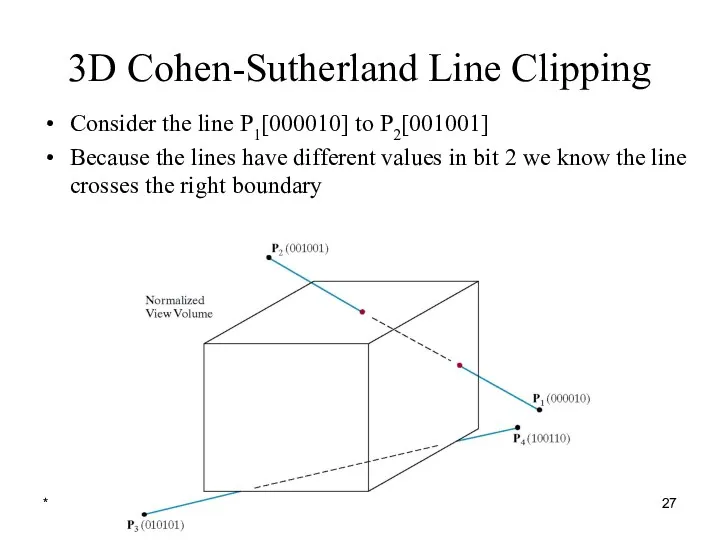
- 27. * Computer Graphics 3D Cohen-Sutherland Line Clipping Consider the line P1[000010] to P2[001001] Because the lines
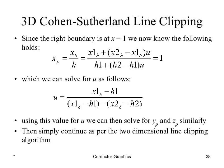
- 28. * Computer Graphics 3D Cohen-Sutherland Line Clipping Since the right boundary is at x = 1
- 30. Скачать презентацию
*
Computer Graphics
Normalized view space
Modeling Transformation
Viewing Transformation
Lighting & Shading
3D-Clipping
Projection
Scan conversion, Hiding
Primitives
Image
Object space
World
*
Computer Graphics
Normalized view space
Modeling Transformation
Viewing Transformation
Lighting & Shading
3D-Clipping
Projection
Scan conversion, Hiding
Primitives
Image
Object space
World
Contents
Introduction
Clipping Volume
Clipping Strategies
Clipping Algorithm
Contents
Introduction
Clipping Volume
Clipping Strategies
Clipping Algorithm
*
Computer Graphics
3D Clipping
Just like the case in two dimensions, clipping removes
*
Computer Graphics
3D Clipping
Just like the case in two dimensions, clipping removes
*
Computer Graphics
3D Clipping
Discarding objects that cannot possibly be seen involves comparing
*
Computer Graphics
3D Clipping
Discarding objects that cannot possibly be seen involves comparing
*
Computer Graphics
3D Clipping
Objects that are partially within the viewing volume need
*
Computer Graphics
3D Clipping
Objects that are partially within the viewing volume need

Contents
Introduction
Clipping Volume
Clipping Strategies
Clipping Algorithm
Contents
Introduction
Clipping Volume
Clipping Strategies
Clipping Algorithm
*
Computer Graphics
The Clipping Volume
In case of Parallel projections the infinite Parallelepiped
*
Computer Graphics
The Clipping Volume
In case of Parallel projections the infinite Parallelepiped
*
Computer Graphics
The Clipping Volume
In case of Perspective projections the semi Infinite
*
Computer Graphics
The Clipping Volume
In case of Perspective projections the semi Infinite
*
Computer Graphics
The Clipping Volume
After the perspective transformation is complete the frustum
*
Computer Graphics
The Clipping Volume
After the perspective transformation is complete the frustum

Contents
Introduction
Clipping Volume
Clipping Strategies
Clipping Algorithm
Contents
Introduction
Clipping Volume
Clipping Strategies
Clipping Algorithm
*
Computer Graphics
Clipping Strategies
Because of the extraordinary computational effort required, two types
*
Computer Graphics
Clipping Strategies
Because of the extraordinary computational effort required, two types
*
Computer Graphics
Clipping Strategies
The canonical view volume for parallel projection is the
*
Computer Graphics
Clipping Strategies
The canonical view volume for parallel projection is the
*
Computer Graphics
Clipping Strategies
The canonical view volume for perspective projection is the
*
Computer Graphics
Clipping Strategies
The canonical view volume for perspective projection is the
*
Computer Graphics
Clipping Strategies
We perform clipping after the projection transformation and normalizations
*
Computer Graphics
Clipping Strategies
We perform clipping after the projection transformation and normalizations
*
Computer Graphics
Clipping Strategies
The basis of canonical clipping is the fact that
*
Computer Graphics
Clipping Strategies
The basis of canonical clipping is the fact that
Contents
Introduction
Clipping Volume
Clipping Strategies
Clipping Algorithm
Contents
Introduction
Clipping Volume
Clipping Strategies
Clipping Algorithm
*
Computer Graphics
Clipping Algorithms
3D clipping algorithms are direct adaptation of 2D clipping
*
Computer Graphics
Clipping Algorithms
3D clipping algorithms are direct adaptation of 2D clipping
*
Computer Graphics
3D Cohen-Sutherland Line Clipping
Similar to the case in two dimensions,
*
Computer Graphics
3D Cohen-Sutherland Line Clipping
Similar to the case in two dimensions,
*
Computer Graphics
3D Cohen-Sutherland Line Clipping
*
Computer Graphics
3D Cohen-Sutherland Line Clipping
*
Computer Graphics
3D Cohen-Sutherland Line Clipping
Now we use a 6 bit out
*
Computer Graphics
3D Cohen-Sutherland Line Clipping
Now we use a 6 bit out
*
Computer Graphics
3D Cohen-Sutherland Line Clipping
CASE – I Assigning region codes to
*
Computer Graphics
3D Cohen-Sutherland Line Clipping
CASE – I Assigning region codes to
*
Computer Graphics
3D Cohen-Sutherland Line Clipping
CASE – II Assigning region codes to
*
Computer Graphics
3D Cohen-Sutherland Line Clipping
CASE – II Assigning region codes to
*
Computer Graphics
3D Cohen-Sutherland Line Clipping
To clip lines we first label all
*
Computer Graphics
3D Cohen-Sutherland Line Clipping
To clip lines we first label all
*
Computer Graphics
3D Cohen-Sutherland Line Clipping
*
Computer Graphics
3D Cohen-Sutherland Line Clipping
*
Computer Graphics
3D Cohen-Sutherland Line Clipping
For clipping equations for three dimensional line
*
Computer Graphics
3D Cohen-Sutherland Line Clipping
For clipping equations for three dimensional line
*
Computer Graphics
3D Cohen-Sutherland Line Clipping
Consider the line P1[000010] to P2[001001]
Because the
*
Computer Graphics
3D Cohen-Sutherland Line Clipping
Consider the line P1[000010] to P2[001001]
Because the
*
Computer Graphics
3D Cohen-Sutherland Line Clipping
Since the right boundary is at x
*
Computer Graphics
3D Cohen-Sutherland Line Clipping
Since the right boundary is at x
 Задачи и стандарты анализа данных
 Создание своего мини-бота в python
 Технология создания и проведения эффективных мультимедиа-презентаций
 Компьютерная графика. Графический редактор
 Влияние интернета на культуру речи
 Решение задач ЕГЭ типа В12
 DS программирование. Циклы while и for
 6 кроків для створення власного логотипу
 Знакомство с графическим оператором DRAW
 Информационные процессы. Информационные системы и технологии
 Help us find the way to the right
 Разновидности объектов и их классификация
 Миниатюра аватара
 Методическая разработка для 7 класса
 Основы языка SQL
 Безпека в інтернеті
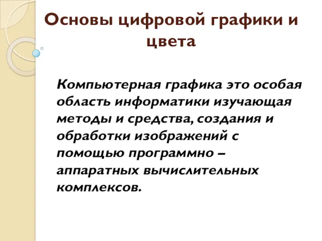 Основы цифровой графики и цвета
 Композиция презентации
 Структуры данных
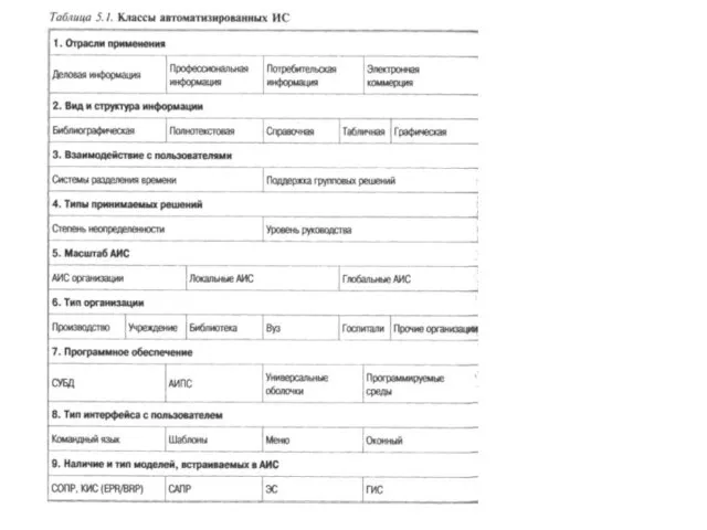 Классификация баз данных по моделям данных. Определение АИС
 двумерные массивы
 Основы реляционной алгебры
 Введение в СУБД ORACLE. Лекция 1
 Процессор - основное устройство обработки информации
 Визитная карточка
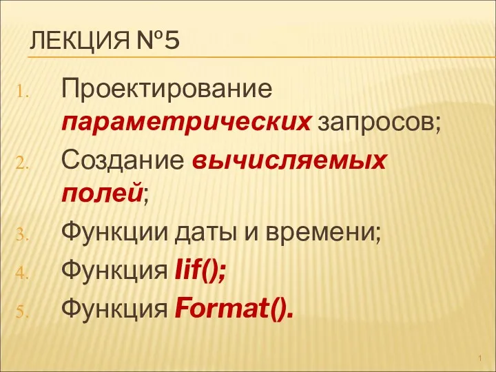 Проектирование параметрических запросов
 Условный оператор IF и оператор выбора CASE [Turbo Pascal]
 Информационное право