- Getting more physical in Call of Duty

Содержание
- 2. Black Ops: shading model Diffuse response Direct: analytical lights Indirect: lightmaps, light probes Lambertian BRDF Specular
- 3. Black Ops: Microfacet BRDF Based on Cook-Torrance: * pl = point light
- 4. Black Ops: normal distribution function Blinn-Phong: Energy conserving Physically plausible stretchy highlights Cheaper replacement for Beckmann
- 5. Black Ops: reflectance function Schlick-Fresnel: rf0: base reflectance (specular color)
- 6. Black Ops: visibility function Schlick-Smith: Compared favorably to: No visibility V(l, v, h) = 1 Cook-Torrance
- 7. Black Ops: environment map normalization Method to “fit” the environment map’s reflection to varying lighting conditions
- 8. Black Ops: normalization algorithm Offline: env_sh9 = capture_sh9(env_pos); env_average_irradiance = env_sh9[0]; for_each (texel in environment map)
- 9. Black Ops: environment map pre-filtering Offline, CubeMapGen Angular Gaussian filter Edge fixup Pixel shader selects mip
- 10. Black Ops: environment map “Fresnel” More than just Fresnel, included shadowing-masking factor Early attempt at deriving
- 11. Getting More Physical in Call of Duty: Black Ops II Direct Specular Very happy with the
- 12. Environment map normalization: problem Average irradiance: poor choice for normalization Light probe Lightmap ?
- 13. Environment map normalization: new idea Normalize with irradiance Can’t bake normalization offline Pass environment map’s directional
- 14. Improved normalization algorithm Offline: env_sh9 = capture_sh9(env_pos); Vertex Shader: env_irradiance = eval_sh(env_sh9, vertex_normal); Pixel Shader: env_color
- 15. Environment map normalization: old method Lightmap Vertex bake Light probe
- 16. Environment map normalization: new method Lightmap Vertex bake Light probe
- 17. Improved environment map pre-filtering Customized CubeMapGen with cosine power filter Concurrent work with Sébastien Lagarde Each
- 18. Environment map pre-filtering: old method gloss 0.0 gloss 1.0 gloss 0.5 sun hotspot
- 19. Environment map pre-filtering: new method gloss 0.0 gloss 1.0 gloss 0.5 sun hotspot
- 20. Environment lighting: ground truth Environment lighting integral
- 21. Environment lighting: split approximation Split the integral: easier to calculate the parts separately Environment map filtering
- 22. Environment BRDF: reflectance interpolation From the Fresnel formulation: rf0 = 0 rf0 = 1
- 23. Numerical integration in Mathematica Plotted two sets of ground-truth curves for rf0 = 0 and rf0
- 24. Approximate curves: accurate rf0 = 1 rf0 = 0 * HLSL expressions in the course notes
- 25. Approximate curves: cheaper rf0 = 1 rf0 = 0 * HLSL expressions in the course notes
- 26. Focus on rf0 = 0.04 Needed faster approximations We had a special-case “simple” material (dielectric only)
- 27. Approximate curves: rf0 = 0.04 float a004(float g, float NoV) { float t = min(0.475 *
- 28. Final approximation float a0r(float g, float NoV) { return (a004(g, NoV) - a1vf(g) * 0.04) /
- 29. Environment BRDF: old method
- 30. Environment BRDF: new method
- 31. Acknowledgments Naty Hoffman Marc Olano Jorge Jimenez Sébastien Lagarde Stephen Hill & Stephen McAuley The team
- 32. We are hiring You can find a list of our open positions at www.activisionblizzard.com/careers. Here is
- 33. Bonus slides
- 34. Black Ops II: new Fresnel approximation Used Mathematica to fit candidate curves
- 36. Скачать презентацию
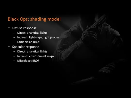
Black Ops: shading model
Diffuse response
Direct: analytical lights
Indirect: lightmaps, light probes
Lambertian BRDF
Specular
Black Ops: shading model
Diffuse response
Direct: analytical lights
Indirect: lightmaps, light probes
Lambertian BRDF
Specular
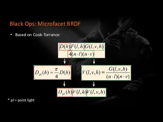
Black Ops: Microfacet BRDF
Based on Cook-Torrance:
* pl = point light
Black Ops: Microfacet BRDF
Based on Cook-Torrance:
* pl = point light
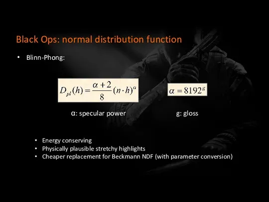
Black Ops: normal distribution function
Blinn-Phong:
Energy conserving
Physically plausible stretchy highlights
Cheaper replacement for
Black Ops: normal distribution function
Blinn-Phong:
Energy conserving
Physically plausible stretchy highlights
Cheaper replacement for
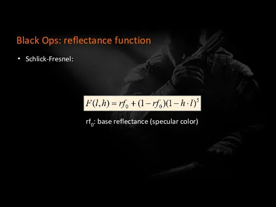
Black Ops: reflectance function
Schlick-Fresnel:
rf0: base reflectance (specular color)
Black Ops: reflectance function
Schlick-Fresnel:
rf0: base reflectance (specular color)
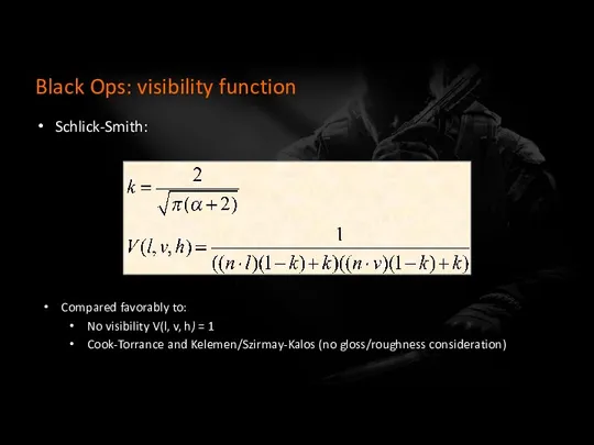
Black Ops: visibility function
Schlick-Smith:
Compared favorably to:
No visibility V(l, v, h) =
Black Ops: visibility function
Schlick-Smith:
Compared favorably to:
No visibility V(l, v, h) =
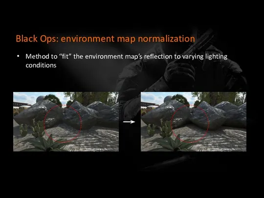
Black Ops: environment map normalization
Method to “fit” the environment map’s reflection
Black Ops: environment map normalization
Method to “fit” the environment map’s reflection
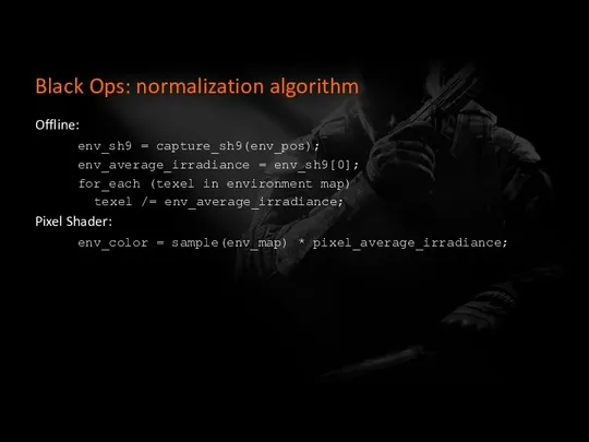
Black Ops: normalization algorithm
Offline:
env_sh9 = capture_sh9(env_pos);
env_average_irradiance = env_sh9[0];
for_each (texel in environment
Black Ops: normalization algorithm
Offline:
env_sh9 = capture_sh9(env_pos);
env_average_irradiance = env_sh9[0];
for_each (texel in environment
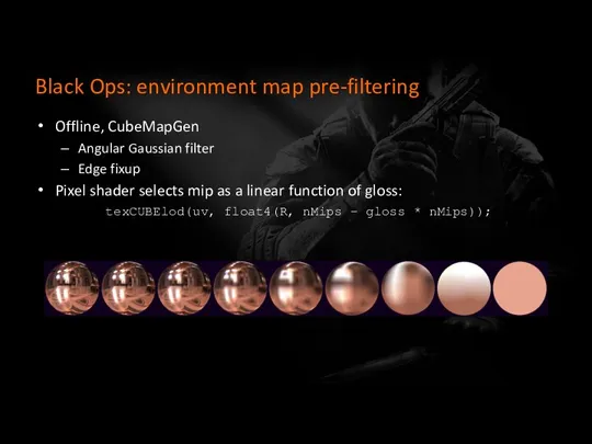
Black Ops: environment map pre-filtering
Offline, CubeMapGen
Angular Gaussian filter
Edge fixup
Pixel shader selects
Black Ops: environment map pre-filtering
Offline, CubeMapGen
Angular Gaussian filter
Edge fixup
Pixel shader selects
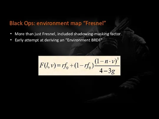
Black Ops: environment map “Fresnel”
More than just Fresnel, included shadowing-masking factor
Early
Black Ops: environment map “Fresnel”
More than just Fresnel, included shadowing-masking factor
Early
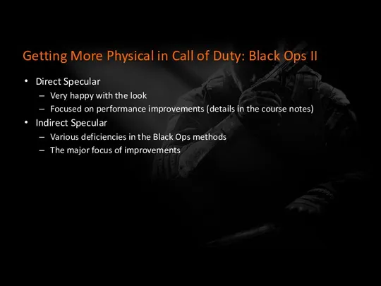
Getting More Physical in Call of Duty: Black Ops II
Direct Specular
Very
Getting More Physical in Call of Duty: Black Ops II
Direct Specular
Very
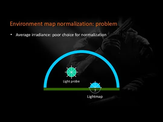
Environment map normalization: problem
Average irradiance: poor choice for normalization
Light probe
Lightmap
?
Environment map normalization: problem
Average irradiance: poor choice for normalization
Light probe
Lightmap
?
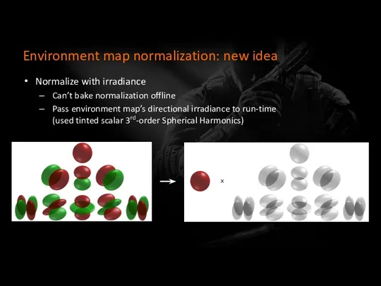
Environment map normalization: new idea
Normalize with irradiance
Can’t bake normalization offline
Pass environment
Environment map normalization: new idea
Normalize with irradiance
Can’t bake normalization offline
Pass environment
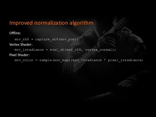
Improved normalization algorithm
Offline:
env_sh9 = capture_sh9(env_pos);
Vertex Shader:
env_irradiance = eval_sh(env_sh9, vertex_normal);
Pixel Shader:
env_color =
Improved normalization algorithm
Offline:
env_sh9 = capture_sh9(env_pos);
Vertex Shader:
env_irradiance = eval_sh(env_sh9, vertex_normal);
Pixel Shader:
env_color =
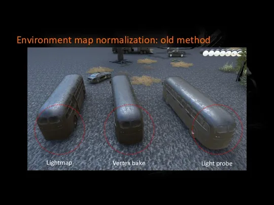
Environment map normalization: old method
Lightmap
Vertex bake
Light probe
Environment map normalization: old method
Lightmap
Vertex bake
Light probe
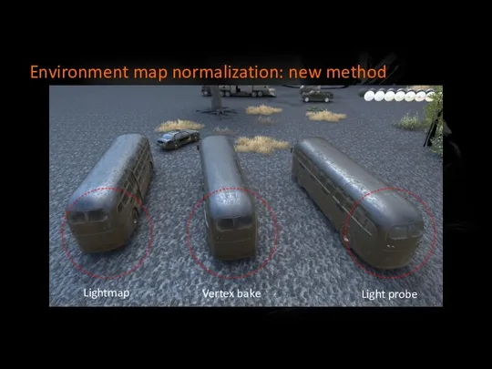
Environment map normalization: new method
Lightmap
Vertex bake
Light probe
Environment map normalization: new method
Lightmap
Vertex bake
Light probe
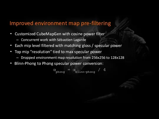
Improved environment map pre-filtering
Customized CubeMapGen with cosine power filter
Concurrent work with
Improved environment map pre-filtering
Customized CubeMapGen with cosine power filter
Concurrent work with
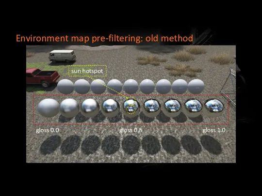
Environment map pre-filtering: old method
gloss 0.0
gloss 1.0
gloss 0.5
sun hotspot
Environment map pre-filtering: old method
gloss 0.0
gloss 1.0
gloss 0.5
sun hotspot
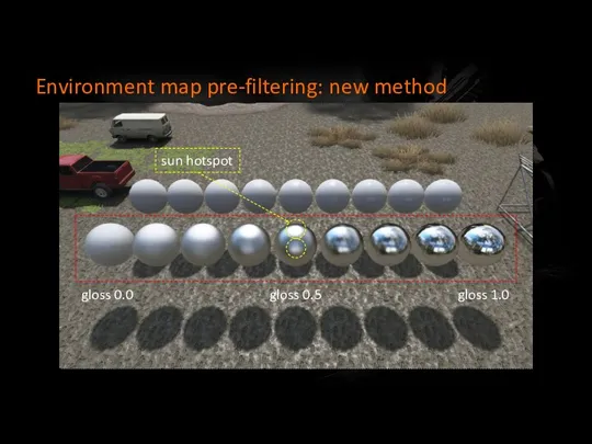
Environment map pre-filtering: new method
gloss 0.0
gloss 1.0
gloss 0.5
sun hotspot
Environment map pre-filtering: new method
gloss 0.0
gloss 1.0
gloss 0.5
sun hotspot
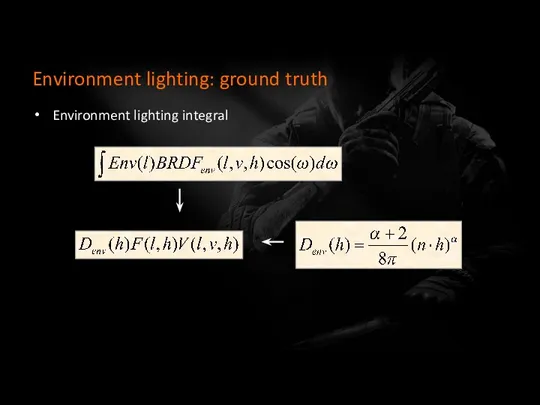
Environment lighting: ground truth
Environment lighting integral
Environment lighting: ground truth
Environment lighting integral
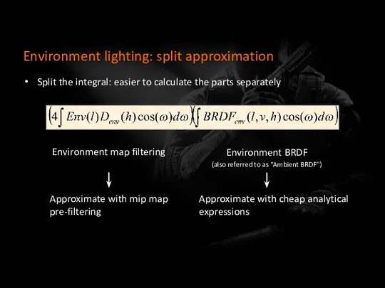
Environment lighting: split approximation
Split the integral: easier to calculate the parts
Environment lighting: split approximation
Split the integral: easier to calculate the parts
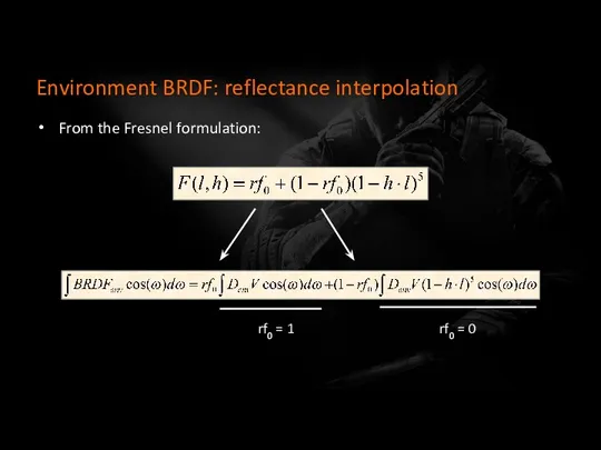
Environment BRDF: reflectance interpolation
From the Fresnel formulation:
rf0 = 0
rf0 = 1
Environment BRDF: reflectance interpolation
From the Fresnel formulation:
rf0 = 0
rf0 = 1
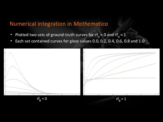
Numerical integration in Mathematica
Plotted two sets of ground-truth curves for rf0
Numerical integration in Mathematica
Plotted two sets of ground-truth curves for rf0
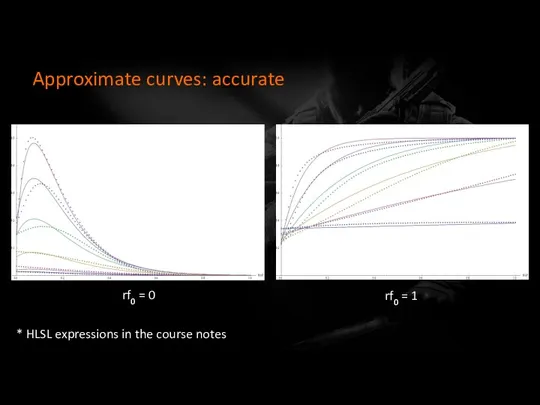
Approximate curves: accurate
rf0 = 1
rf0 = 0
* HLSL expressions in the
Approximate curves: accurate
rf0 = 1
rf0 = 0
* HLSL expressions in the
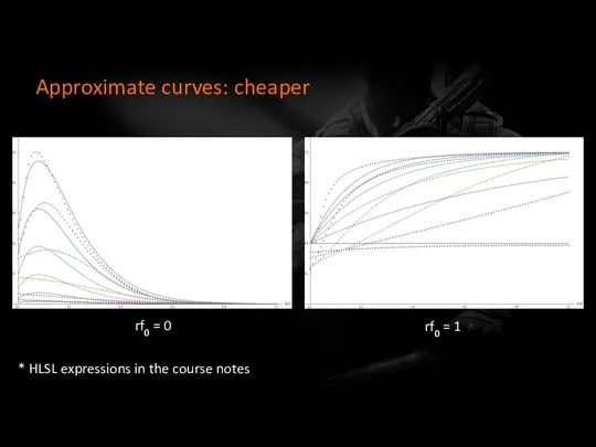
Approximate curves: cheaper
rf0 = 1
rf0 = 0
* HLSL expressions in the
Approximate curves: cheaper
rf0 = 1
rf0 = 0
* HLSL expressions in the
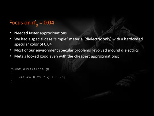
Focus on rf0 = 0.04
Needed faster approximations
We had a special-case “simple”
Focus on rf0 = 0.04
Needed faster approximations
We had a special-case “simple”
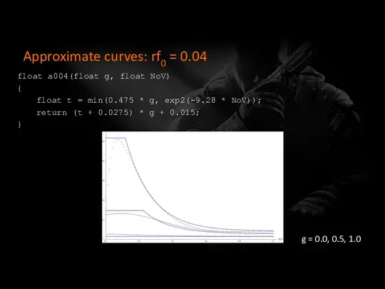
Approximate curves: rf0 = 0.04
float a004(float g, float NoV)
{
float t =
Approximate curves: rf0 = 0.04
float a004(float g, float NoV)
{
float t =
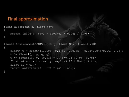
Final approximation
float a0r(float g, float NoV)
{
return (a004(g, NoV) - a1vf(g) *
Final approximation
float a0r(float g, float NoV)
{
return (a004(g, NoV) - a1vf(g) *
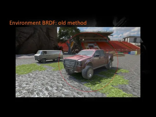
Environment BRDF: old method
Environment BRDF: old method
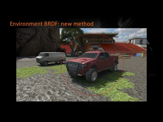
Environment BRDF: new method
Environment BRDF: new method
Acknowledgments
Naty Hoffman
Marc Olano
Jorge Jimenez
Sébastien Lagarde
Stephen Hill & Stephen McAuley
The team at
Acknowledgments
Naty Hoffman
Marc Olano
Jorge Jimenez
Sébastien Lagarde
Stephen Hill & Stephen McAuley
The team at
We are hiring
You can find a list of our open positions
We are hiring
You can find a list of our open positions
Bonus slides
Bonus slides
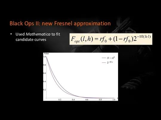
Black Ops II: new Fresnel approximation
Used Mathematica to fit candidate curves
Black Ops II: new Fresnel approximation
Used Mathematica to fit candidate curves
 Мобильная электронная подпись (МЭП). Инструмент подписания электронных документов
 Автоматизированные системы различного назначения, примеры их использования.. Лекция 16
 Какими я вижу компьютеры будущего
 Проектирование в KOMANDOR Designer
 Вероятностный подход к измерению информации. Лекция 3
 WEB-Index: Аудитория интернет-проектов
 Хранение и обработка информации в базах данных
 Service bulletin. Appendix A. S/W Guide
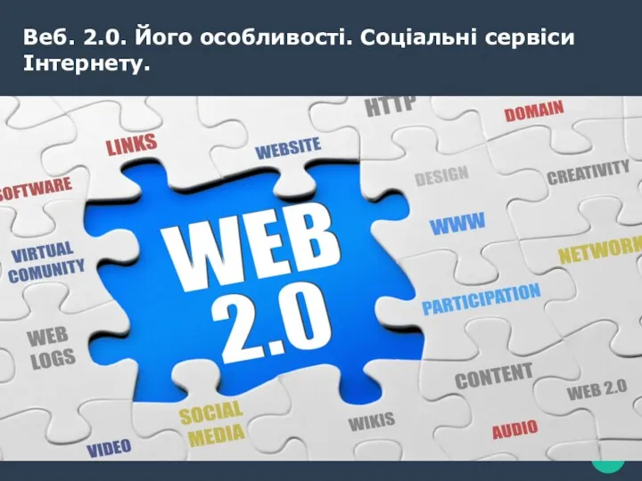 Веб. 2.0. Його особливості. Соціальні сервіси Інтернету
 CCSv6 Tips & Tricks
 План урока по теме Интернет. Поиск информации в компьютерных сетях
 Информация: формы, измерение, количество и качество
 Проект обмена данными ЕХБ дилеров
 Технология монтажа и обслуживания телекоммуникационных систем с коммутацией пакетов. Тема 1.2
 Промышленные сети
 Оптимизация нелинейных систем
 Представление числовой информации с помощью систем счисления
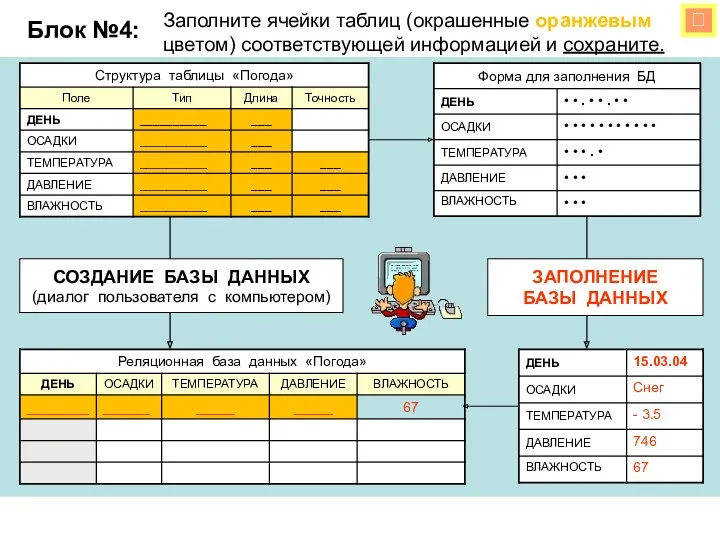 9 класс. Урок на тему: Условия выбора и сложные логические выражения
 Первое поколение ЭВМ
 Возможности динамических (электронных) таблиц
 Хранение информационных объектов различных видов на различных цифровых носителях
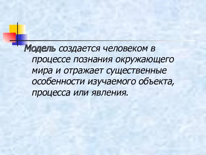 Классификация моделей. Исследование физической модели
 Инструменты для распознавания текстов и системы компьютерного перевода. Оценка количественных параметров текстовых документов
 История развития компьютеров
 Логическое программирование (Prolog)
 Конфигурирование и проверка конфигурирования перераспределения. (Модуль 5, Лекция 2.1)
 Глобальна комп’ютерна мережа Інтернет
 Методи та системи паралельного програмування