- Modeling and Solving Constraints. Basic Idea

Содержание
- 2. Basic Idea Constraints are used to simulate joints, contact, and collision. We need to solve the
- 3. Overview Constraint Formulas Jacobians, Lagrange Multipliers Modeling Constraints Joints, Motors, Contact Building a Constraint Solver Sequential
- 4. Constraint Types Contact and Friction
- 5. Constraint Types Ragdolls
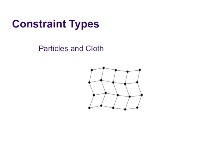
- 6. Constraint Types Particles and Cloth
- 7. Show Me the Demo!
- 8. Bead on a 2D Rigid Wire Implicit Curve Equation: This is the position constraint.
- 9. How does it move? The normal vector is perpendicular to the velocity.
- 10. Enter The Calculus Position Constraint: Velocity Constraint: If C is zero, then its time derivative is
- 11. Velocity Constraint Velocity constraints define the allowed motion. Next we’ll show that velocity constraints depend linearly
- 12. The Jacobian Due to the chain rule the velocity constraint has a special structure: J is
- 13. The Jacobian The Jacobian is perpendicular to the velocity.
- 14. Constraint Force Assume the wire is frictionless. What is the force between the wire and the
- 15. Lagrange Multiplier Intuitively the constraint force Fc is parallel to the normal vector. Direction known. Magnitude
- 16. Lagrange Multiplier The Lagrange Multiplier (lambda) is the constraint force signed magnitude. We use a constraint
- 17. Jacobian as a CoordinateTransform Similar to a rotation matrix. Except it is missing a couple rows.
- 18. Velocity Transform v Cartesian Space Velocity Constraint Space Velocity
- 19. Force Transform Constraint Space Force Cartesian Space Force
- 20. Refresher: Work and Power Work = Force times Distance Work has units of Energy (Joules) Power
- 21. Principle of Virtual Work Principle: constraint forces do no work. Proof (compute the power): The power
- 22. Constraint Quantities Position Constraint Velocity Constraint Jacobian Lagrange Multiplier
- 23. Why all the Painful Abstraction? We want to put all constraints into a common form for
- 24. Addendum: Modeling Time Dependence Some constraints, like motors, have prescribed motion. This is represented by time
- 25. Example: Distance Constraint y x L Position: Velocity: Jacobian: Velocity Bias: particle
- 26. Gory Details
- 27. Computing the Jacobian At first, it is not easy to compute the Jacobian. It gets easier
- 28. A Recipe for J Use geometry to write C. Differentiate C with respect to time. Isolate
- 29. Constraint Potpourri Joints Motors Contact Restitution Friction
- 30. Joint: Distance Constraint y x v
- 31. Motors A motor is a constraint with limited force (torque). Example A Wheel Note: this constraint
- 32. Velocity Only Motors Example Usage: A wheel that spins at a constant rate. We don’t care
- 33. Inequality Constraints So far we’ve looked at equality constraints (because they are simpler). Inequality constraints are
- 34. Inequality Constraints The corresponding velocity constraint: If Else skip constraint enforce:
- 35. Inequality Constraints Force Limits: Inequality constraints don’t suck.
- 36. Contact Constraint Non-penetration. Restitution: bounce Friction: sliding, sticking, and rolling
- 37. Non-Penetration Constraint body 2 body 1 (separation)
- 38. Non-Penetration Constraint J Handy Identities
- 39. Restitution Relative normal velocity Adding bounce as a velocity bias Velocity Reflection
- 40. Friction Constraint Friction is like a velocity-only motor. The target velocity is zero. J
- 41. Friction Constraint The friction force is limited by the normal force. Coulomb’s Law: In 2D: 3D
- 42. Constraints Solvers We have a bunch of constraints. We have unknown constraint forces. We need to
- 43. Constraint Solver Types Global Solvers (slow) Iterative Solvers (fast)
- 44. Solving a Chain λ1 λ2 λ3 Global: solve for λ1, λ2, and λ3 simultaneously. Iterative: while
- 45. Sequential Impulses (SI) An iterative solver. SI applies impulses at each constraint to correct the velocity
- 46. Why Impulses? Easier to deal with friction and collision. Lets us work with velocity rather than
- 47. Sequential Impulses Step1: Integrate applied forces, yielding tentative velocities. Step2: Apply impulses sequentially for all constraints,
- 48. Step 1: Newton’s Law We separate applied forces and constraint forces. mass matrix
- 49. Step 1: Mass Matrix Particle Rigid Body May involve multiple particles/bodies.
- 50. Step 1: Applied Forces Applied forces are computed according to some law. Gravity: F = mg
- 51. Step 1 : Integrate Applied Forces Euler’s Method for all bodies. This new velocity tends to
- 52. Step 2: Constraint Impulse The constraint impulse is just the time step times the constraint force.
- 53. Step 2: Impulse-Momentum Newton’s Law for impulses: In other words:
- 54. Step 2: Computing Lambda For each constraint, solve these for λ: Newton’s Law: Virtual Work: Velocity
- 55. Step 2: Impulse Solution The scalar mC is the effective mass seen by the constraint impulse:
- 56. Step 2: Velocity Update Now that we solved for lambda, we can use it to update
- 57. Step 2: Iteration Loop over all constraints until you are done: - Fixed number of iterations.
- 58. Step 3: Integrate Positions Use the new velocity to integrate all body positions (and orientations): This
- 59. Extensions to Step 2 Handle position drift. Handle force limits. Handle inequality constraints. Warm starting.
- 60. Handling Position Drift Velocity constraints are not obeyed precisely. Joints will fall apart.
- 61. Baumgarte Stabilization Feed the position error back into the velocity constraint. New velocity constraint: Bias factor:
- 62. Baumgarte Stabilization What is the solution to this? First-order differential equation …
- 63. Answer
- 64. Tuning the Bias Factor If your simulation has instabilities, set the bias factor to zero and
- 65. Handling Force Limits First, convert force limits to impulse limits.
- 66. Handling Impulse Limits Clamping corrective impulses: Is it really that simple? Hint: no.
- 67. How to Clamp Each iteration computes corrective impulses. Clamping corrective impulses is wrong! You should clamp
- 68. Example: 2D Inelastic Collision v A Falling Box Global Solution
- 69. Iterative Solution iteration 1 constraint 1 constraint 2 Suppose the corrective impulses are too strong. What
- 70. Iterative Solution iteration 2 To keep the box from bouncing, we need downward corrective impulses. In
- 71. Iterative Solution But clamping the negative corrective impulses wipes them out: This is one way to
- 72. Accumulated Impulses For each constraint, keep track of the total impulse applied. This is the accumulated
- 73. New Clamping Procedure Compute the corrective impulse, but don’t apply it. Make a copy of the
- 74. Handling Inequality Constraints Before iterations, determine if the inequality constraint is active. If it is inactive,
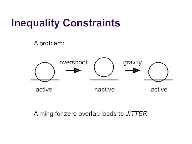
- 75. Inequality Constraints A problem: overshoot active inactive active gravity Aiming for zero overlap leads to JITTER!
- 76. Preventing Overshoot Allow a little bit of penetration (slop). If separation Else Note: the slop will
- 77. Warm Starting Iterative solvers use an initial guess for the lambdas. So save the lambdas from
- 78. Step 1.5 Apply the stored impulses. Use the stored impulses to initialize the accumulated impulses.
- 79. Step 2.5 Store the accumulated impulses.
- 80. Further Reading & Sample Code http://www.gphysics.com/downloads/
- 82. Скачать презентацию
Basic Idea
Constraints are used to simulate joints, contact, and collision.
We need
Basic Idea
Constraints are used to simulate joints, contact, and collision.
We need
Overview
Constraint Formulas
Jacobians, Lagrange Multipliers
Modeling Constraints
Joints, Motors, Contact
Building a Constraint Solver
Sequential Impulses
Overview
Constraint Formulas
Jacobians, Lagrange Multipliers
Modeling Constraints
Joints, Motors, Contact
Building a Constraint Solver
Sequential Impulses
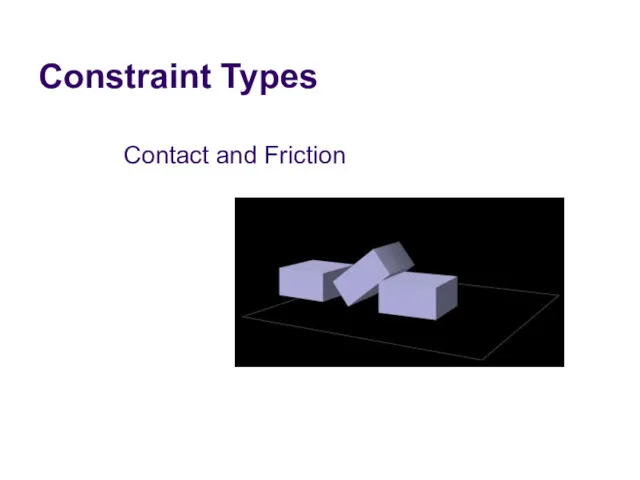
Constraint Types
Contact and Friction
Constraint Types
Contact and Friction
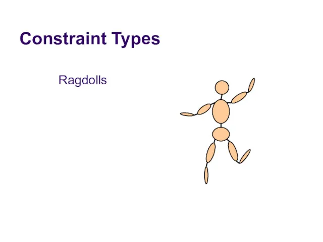
Constraint Types
Ragdolls
Constraint Types
Ragdolls
Constraint Types
Particles and Cloth
Constraint Types
Particles and Cloth
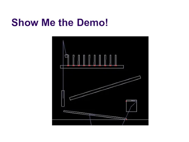
Show Me the Demo!
Show Me the Demo!
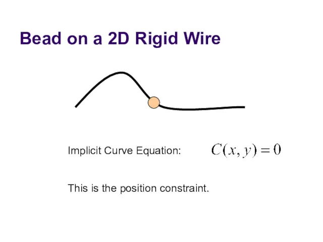
Bead on a 2D Rigid Wire
Implicit Curve Equation:
This is the position
Bead on a 2D Rigid Wire
Implicit Curve Equation:
This is the position
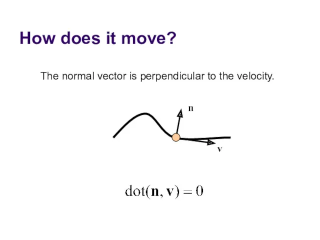
How does it move?
The normal vector is perpendicular to the velocity.
How does it move?
The normal vector is perpendicular to the velocity.
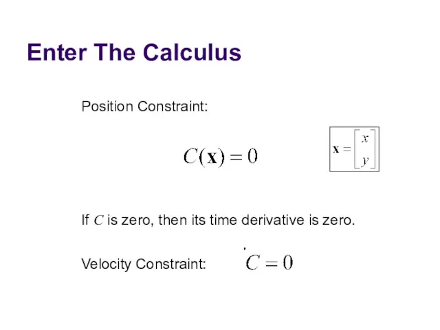
Enter The Calculus
Position Constraint:
Velocity Constraint:
If C is zero, then its time
Enter The Calculus
Position Constraint:
Velocity Constraint:
If C is zero, then its time

Velocity Constraint
Velocity constraints define the allowed motion.
Next we’ll show that velocity
Velocity Constraint
Velocity constraints define the allowed motion.
Next we’ll show that velocity
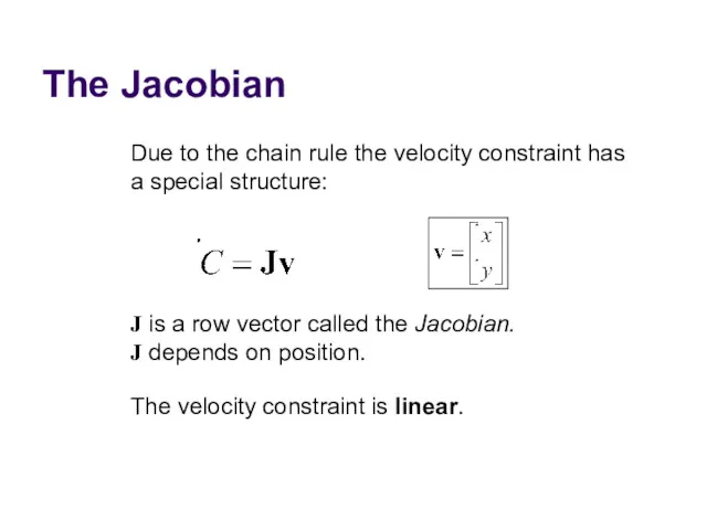
The Jacobian
Due to the chain rule the velocity constraint has a
The Jacobian
Due to the chain rule the velocity constraint has a
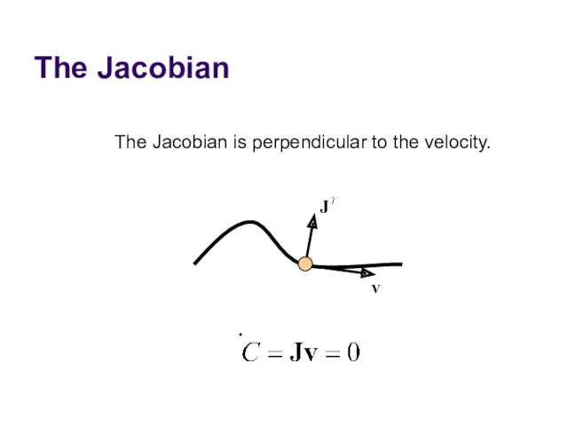
The Jacobian
The Jacobian is perpendicular to the velocity.
The Jacobian
The Jacobian is perpendicular to the velocity.
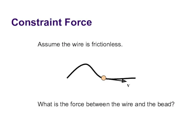
Constraint Force
Assume the wire is frictionless.
What is the force between the
Constraint Force
Assume the wire is frictionless.
What is the force between the
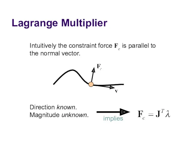
Lagrange Multiplier
Intuitively the constraint force Fc is parallel to the normal
Lagrange Multiplier
Intuitively the constraint force Fc is parallel to the normal
Lagrange Multiplier
The Lagrange Multiplier (lambda) is the constraint force signed magnitude.
We
Lagrange Multiplier
The Lagrange Multiplier (lambda) is the constraint force signed magnitude.
We
Jacobian as a CoordinateTransform
Similar to a rotation matrix.
Except it is missing
Jacobian as a CoordinateTransform
Similar to a rotation matrix.
Except it is missing
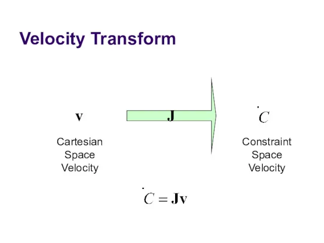
Velocity Transform
v
Cartesian
Space
Velocity
Constraint
Space
Velocity
Velocity Transform
v
Cartesian
Space
Velocity
Constraint
Space
Velocity
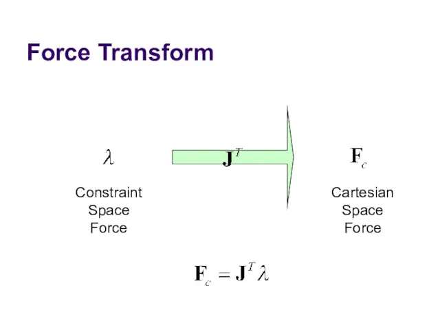
Force Transform
Constraint
Space
Force
Cartesian
Space
Force
Force Transform
Constraint
Space
Force
Cartesian
Space
Force
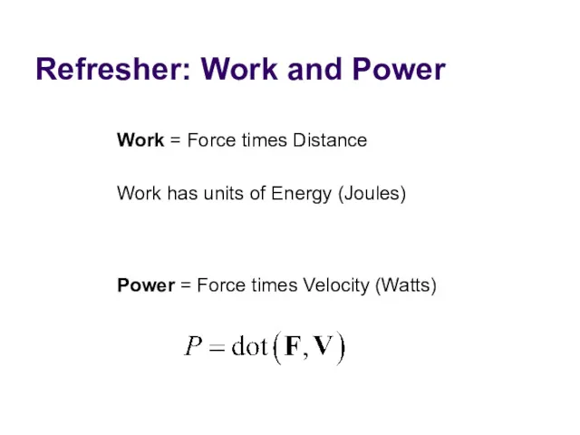
Refresher: Work and Power
Work = Force times Distance
Work has units of
Refresher: Work and Power
Work = Force times Distance
Work has units of
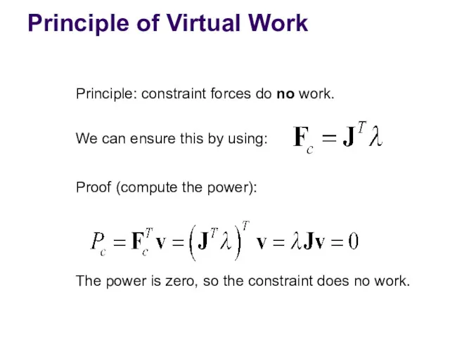
Principle of Virtual Work
Principle: constraint forces do no work.
Proof (compute the
Principle of Virtual Work
Principle: constraint forces do no work.
Proof (compute the
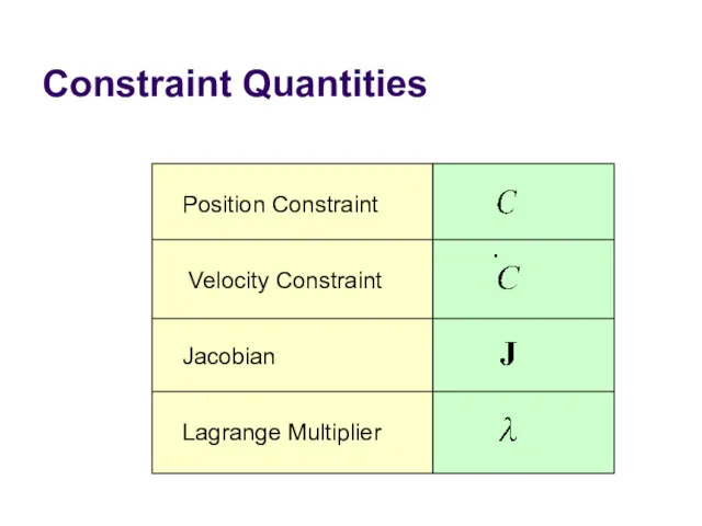
Constraint Quantities
Position Constraint
Velocity Constraint
Jacobian
Lagrange Multiplier
Constraint Quantities
Position Constraint
Velocity Constraint
Jacobian
Lagrange Multiplier

Why all the Painful Abstraction?
We want to put all constraints into
Why all the Painful Abstraction?
We want to put all constraints into
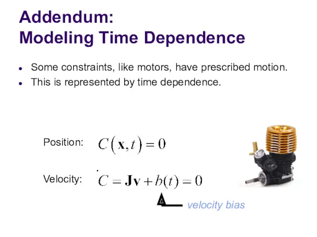
Addendum:
Modeling Time Dependence
Some constraints, like motors, have prescribed motion.
This is represented
Addendum:
Modeling Time Dependence
Some constraints, like motors, have prescribed motion.
This is represented
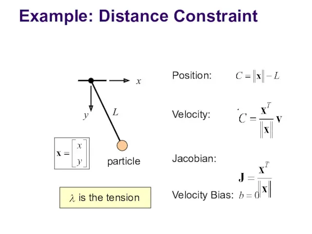
Example: Distance Constraint
y
x
L
Position:
Velocity:
Jacobian:
Velocity Bias:
particle
Example: Distance Constraint
y
x
L
Position:
Velocity:
Jacobian:
Velocity Bias:
particle
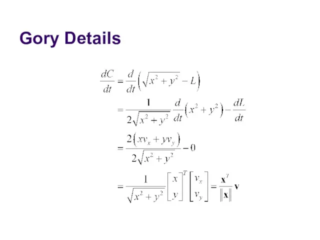
Gory Details
Gory Details
Computing the Jacobian
At first, it is not easy to compute the
Computing the Jacobian
At first, it is not easy to compute the
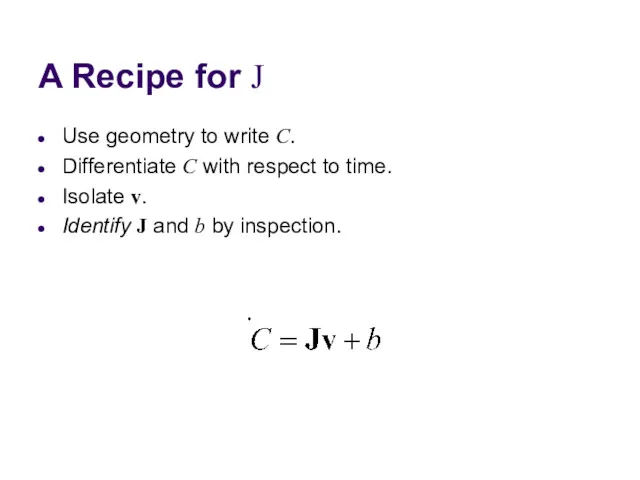
A Recipe for J
Use geometry to write C.
Differentiate C with respect
A Recipe for J
Use geometry to write C.
Differentiate C with respect
Constraint Potpourri
Joints
Motors
Contact
Restitution
Friction
Constraint Potpourri
Joints
Motors
Contact
Restitution
Friction
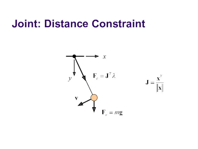
Joint: Distance Constraint
y
x
v
Joint: Distance Constraint
y
x
v
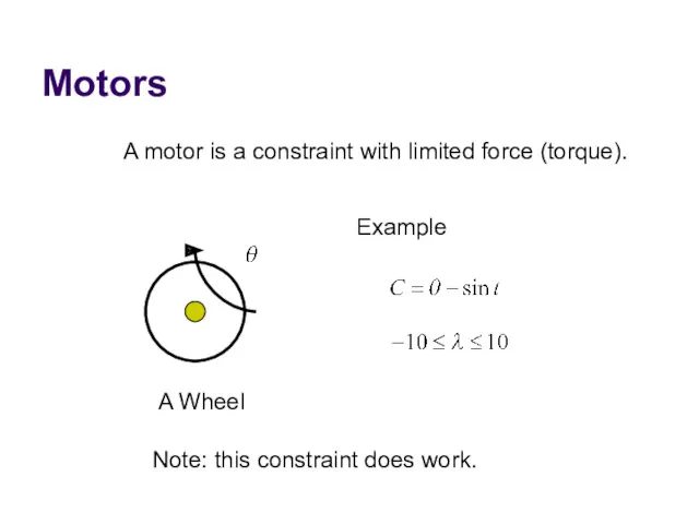
Motors
A motor is a constraint with limited force (torque).
Example
A Wheel
Note: this
Motors
A motor is a constraint with limited force (torque).
Example
A Wheel
Note: this
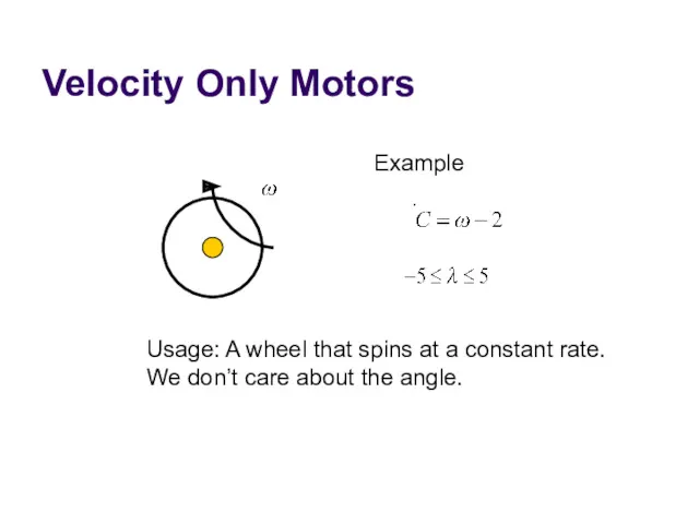
Velocity Only Motors
Example
Usage: A wheel that spins at a constant rate.
We
Velocity Only Motors
Example
Usage: A wheel that spins at a constant rate.
We
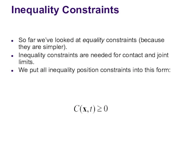
Inequality Constraints
So far we’ve looked at equality constraints (because they are
Inequality Constraints
So far we’ve looked at equality constraints (because they are

Inequality Constraints
The corresponding velocity constraint:
If
Else
skip constraint
enforce:
Inequality Constraints
The corresponding velocity constraint:
If
Else
skip constraint
enforce:
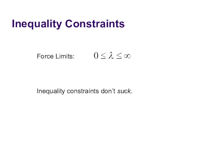
Inequality Constraints
Force Limits:
Inequality constraints don’t suck.
Inequality Constraints
Force Limits:
Inequality constraints don’t suck.
Contact Constraint
Non-penetration.
Restitution: bounce
Friction: sliding, sticking, and rolling
Contact Constraint
Non-penetration.
Restitution: bounce
Friction: sliding, sticking, and rolling
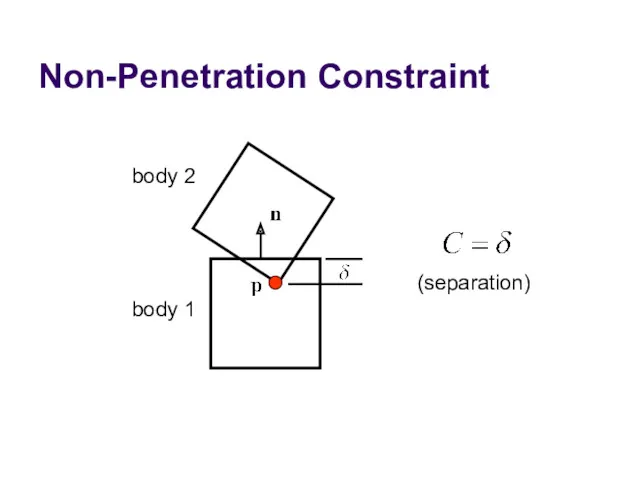
Non-Penetration Constraint
body 2
body 1
(separation)
Non-Penetration Constraint
body 2
body 1
(separation)
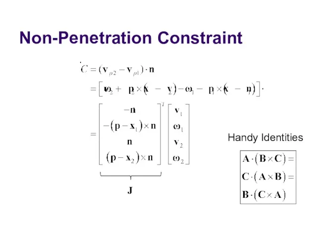
Non-Penetration Constraint
J
Handy Identities
Non-Penetration Constraint
J
Handy Identities
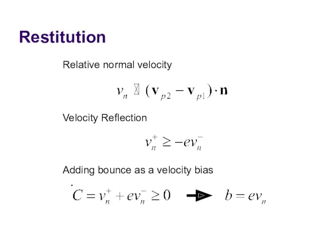
Restitution
Relative normal velocity
Adding bounce as a velocity bias
Velocity Reflection
Restitution
Relative normal velocity
Adding bounce as a velocity bias
Velocity Reflection
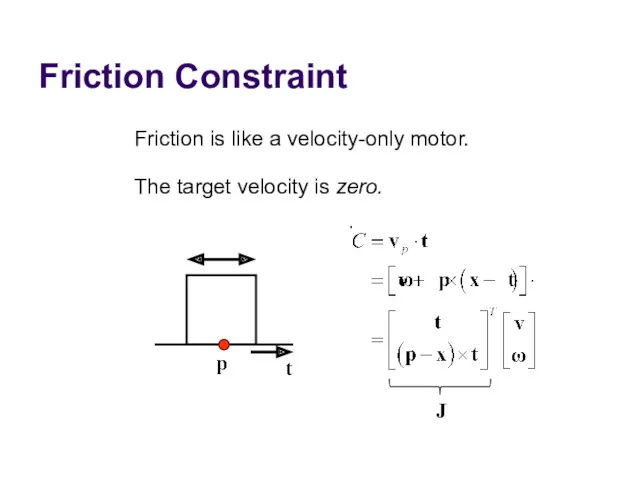
Friction Constraint
Friction is like a velocity-only motor.
The target velocity is zero.
J
Friction Constraint
Friction is like a velocity-only motor.
The target velocity is zero.
J
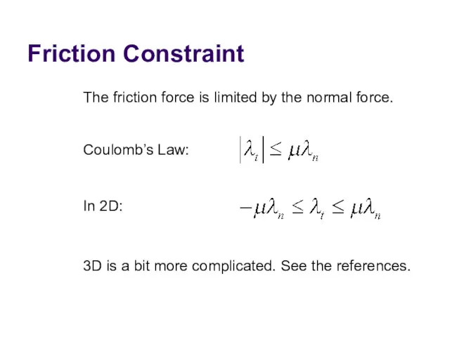
Friction Constraint
The friction force is limited by the normal force.
Coulomb’s Law:
In
Friction Constraint
The friction force is limited by the normal force.
Coulomb’s Law:
In
Constraints Solvers
We have a bunch of constraints.
We have unknown constraint forces.
We
Constraints Solvers
We have a bunch of constraints.
We have unknown constraint forces.
We
Constraint Solver Types
Global Solvers (slow)
Iterative Solvers (fast)
Constraint Solver Types
Global Solvers (slow)
Iterative Solvers (fast)
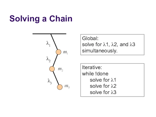
Solving a Chain
λ1
λ2
λ3
Global:
solve for λ1, λ2, and λ3 simultaneously.
Iterative:
while !done
solve for
Solving a Chain
λ1
λ2
λ3
Global:
solve for λ1, λ2, and λ3 simultaneously.
Iterative:
while !done
solve for
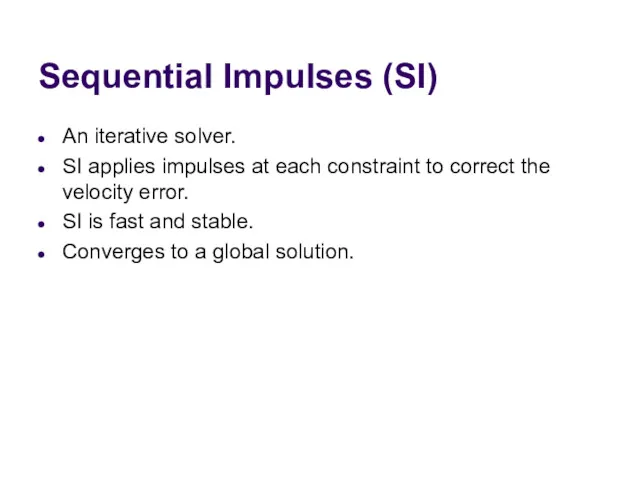
Sequential Impulses (SI)
An iterative solver.
SI applies impulses at each constraint to
Sequential Impulses (SI)
An iterative solver.
SI applies impulses at each constraint to
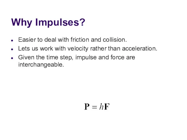
Why Impulses?
Easier to deal with friction and collision.
Lets us work with
Why Impulses?
Easier to deal with friction and collision.
Lets us work with
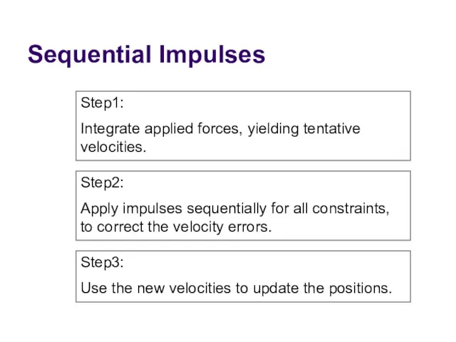
Sequential Impulses
Step1:
Integrate applied forces, yielding tentative velocities.
Step2:
Apply impulses sequentially for all
Sequential Impulses
Step1:
Integrate applied forces, yielding tentative velocities.
Step2:
Apply impulses sequentially for all
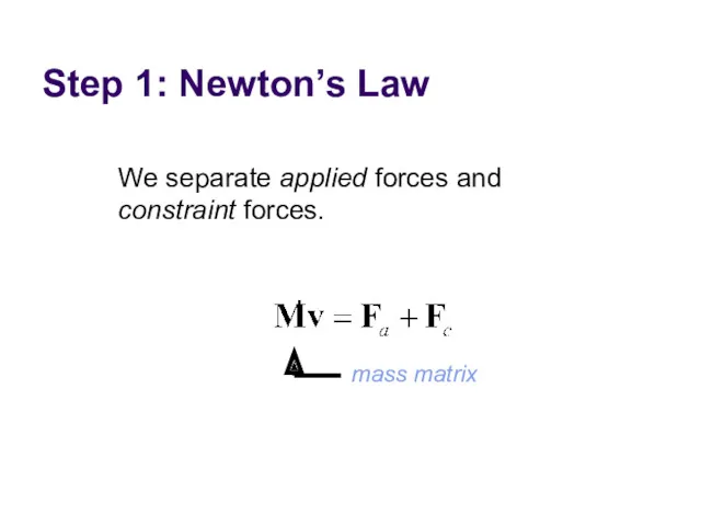
Step 1: Newton’s Law
We separate applied forces and
constraint forces.
mass matrix
Step 1: Newton’s Law
We separate applied forces and
constraint forces.
mass matrix
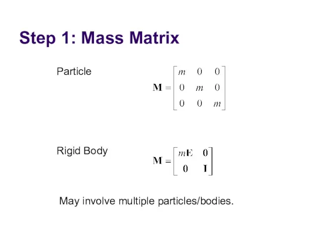
Step 1: Mass Matrix
Particle
Rigid Body
May involve multiple particles/bodies.
Step 1: Mass Matrix
Particle
Rigid Body
May involve multiple particles/bodies.
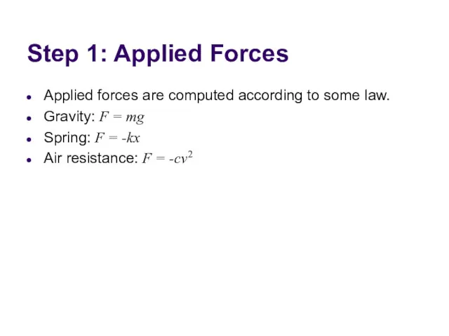
Step 1: Applied Forces
Applied forces are computed according to some law.
Gravity:
Step 1: Applied Forces
Applied forces are computed according to some law.
Gravity:
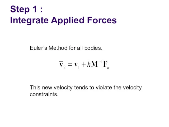
Step 1 :
Integrate Applied Forces
Euler’s Method for all bodies.
This new velocity
Step 1 :
Integrate Applied Forces
Euler’s Method for all bodies.
This new velocity
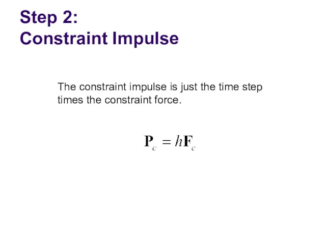
Step 2:
Constraint Impulse
The constraint impulse is just the time step times
Step 2:
Constraint Impulse
The constraint impulse is just the time step times
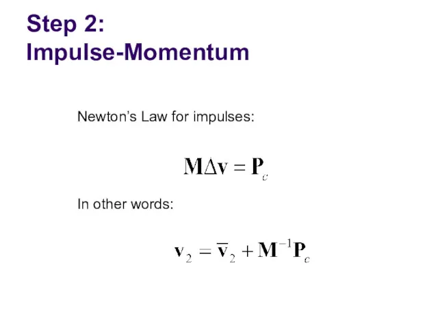
Step 2:
Impulse-Momentum
Newton’s Law for impulses:
In other words:
Step 2:
Impulse-Momentum
Newton’s Law for impulses:
In other words:
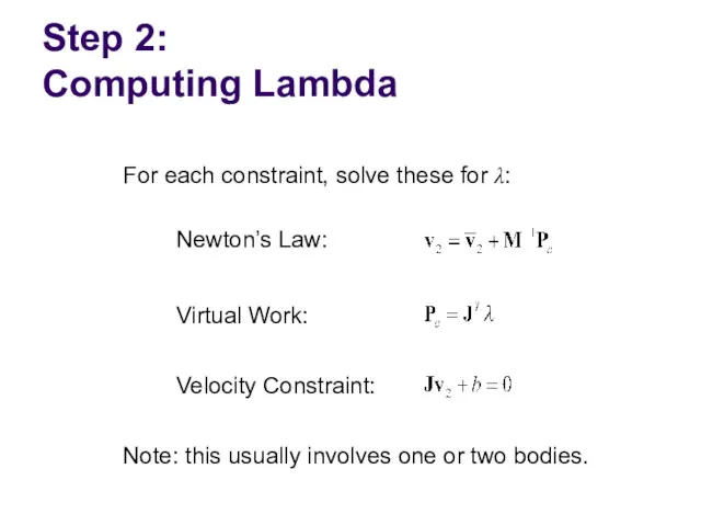
Step 2:
Computing Lambda
For each constraint, solve these for λ:
Newton’s Law:
Virtual Work:
Velocity
Step 2:
Computing Lambda
For each constraint, solve these for λ:
Newton’s Law:
Virtual Work:
Velocity
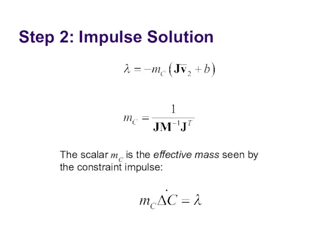
Step 2: Impulse Solution
The scalar mC is the effective mass seen
Step 2: Impulse Solution
The scalar mC is the effective mass seen
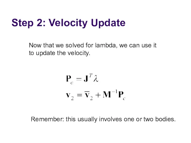
Step 2: Velocity Update
Now that we solved for lambda, we can
Step 2: Velocity Update
Now that we solved for lambda, we can
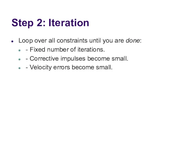
Step 2: Iteration
Loop over all constraints until you are done:
- Fixed
Step 2: Iteration
Loop over all constraints until you are done:
- Fixed
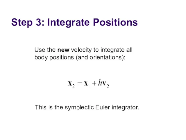
Step 3: Integrate Positions
Use the new velocity to integrate all body
Step 3: Integrate Positions
Use the new velocity to integrate all body
Extensions to Step 2
Handle position drift.
Handle force limits.
Handle inequality constraints.
Warm starting.
Extensions to Step 2
Handle position drift.
Handle force limits.
Handle inequality constraints.
Warm starting.
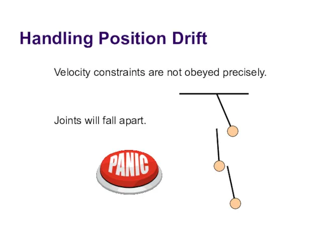
Handling Position Drift
Velocity constraints are not obeyed precisely.
Joints will fall apart.
Handling Position Drift
Velocity constraints are not obeyed precisely.
Joints will fall apart.
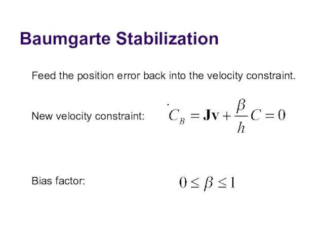
Baumgarte Stabilization
Feed the position error back into the velocity constraint.
New velocity
Baumgarte Stabilization
Feed the position error back into the velocity constraint.
New velocity
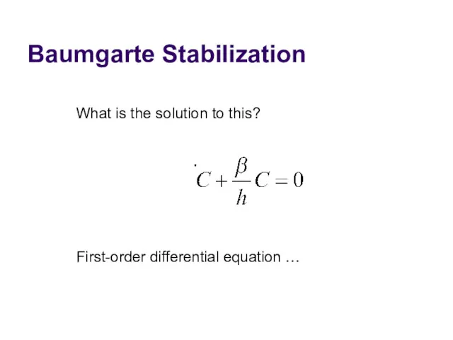
Baumgarte Stabilization
What is the solution to this?
First-order differential equation …
Baumgarte Stabilization
What is the solution to this?
First-order differential equation …
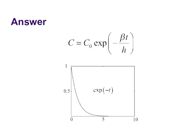
Answer
Answer
Tuning the Bias Factor
If your simulation has instabilities, set the bias
Tuning the Bias Factor
If your simulation has instabilities, set the bias
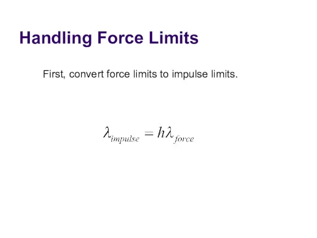
Handling Force Limits
First, convert force limits to impulse limits.
Handling Force Limits
First, convert force limits to impulse limits.
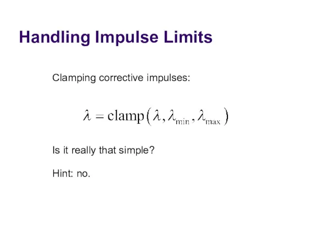
Handling Impulse Limits
Clamping corrective impulses:
Is it really that simple?
Hint: no.
Handling Impulse Limits
Clamping corrective impulses:
Is it really that simple?
Hint: no.
How to Clamp
Each iteration computes corrective impulses.
Clamping corrective impulses is wrong!
You
How to Clamp
Each iteration computes corrective impulses.
Clamping corrective impulses is wrong!
You
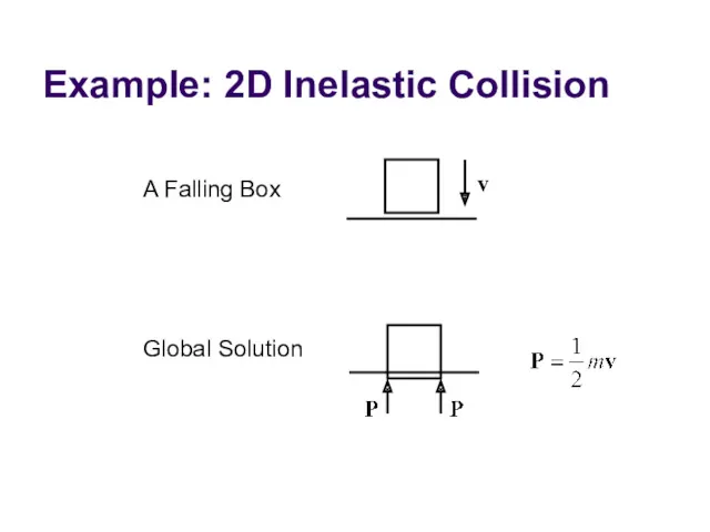
Example: 2D Inelastic Collision
v
A Falling Box
Global Solution
Example: 2D Inelastic Collision
v
A Falling Box
Global Solution
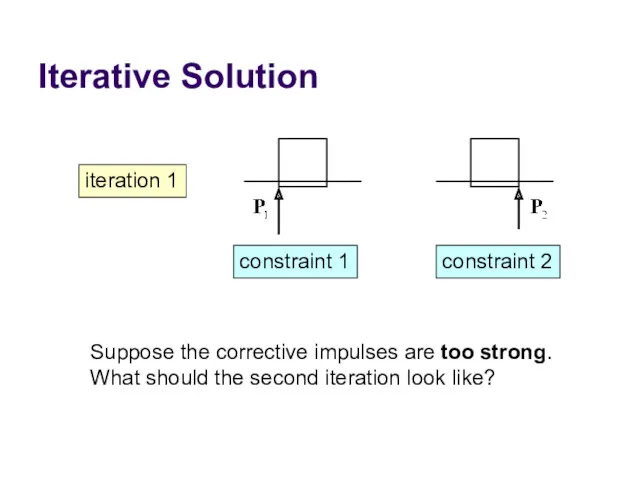
Iterative Solution
iteration 1
constraint 1
constraint 2
Suppose the corrective impulses are too strong.
What
Iterative Solution
iteration 1
constraint 1
constraint 2
Suppose the corrective impulses are too strong.
What
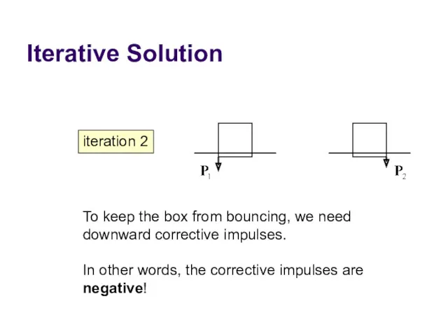
Iterative Solution
iteration 2
To keep the box from bouncing, we need
downward corrective
Iterative Solution
iteration 2
To keep the box from bouncing, we need
downward corrective
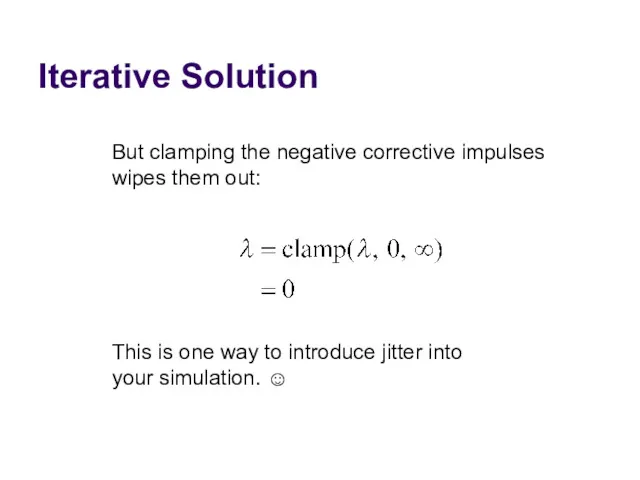
Iterative Solution
But clamping the negative corrective impulses
wipes them out:
This is one
Iterative Solution
But clamping the negative corrective impulses
wipes them out:
This is one
Accumulated Impulses
For each constraint, keep track of the total impulse applied.
This
Accumulated Impulses
For each constraint, keep track of the total impulse applied.
This
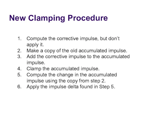
New Clamping Procedure
Compute the corrective impulse, but don’t apply it.
Make a
New Clamping Procedure
Compute the corrective impulse, but don’t apply it.
Make a
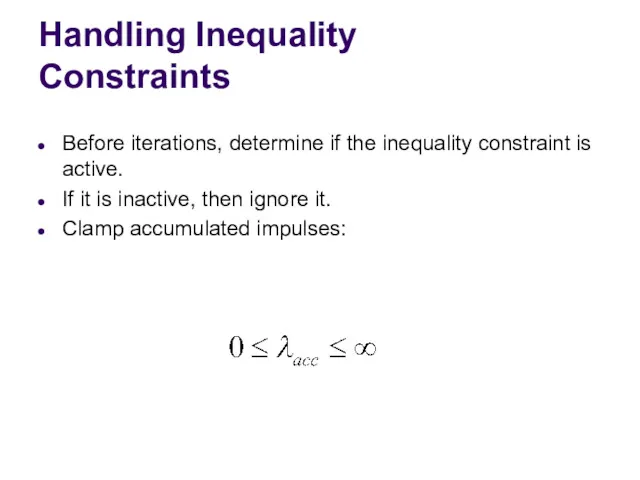
Handling Inequality Constraints
Before iterations, determine if the inequality constraint is active.
If
Handling Inequality Constraints
Before iterations, determine if the inequality constraint is active.
If
Inequality Constraints
A problem:
overshoot
active
inactive
active
gravity
Aiming for zero overlap leads to JITTER!
Inequality Constraints
A problem:
overshoot
active
inactive
active
gravity
Aiming for zero overlap leads to JITTER!
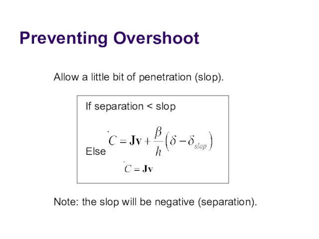
Preventing Overshoot
Allow a little bit of penetration (slop).
If separation < slop
Else
Note:
Preventing Overshoot
Allow a little bit of penetration (slop).
If separation < slop
Else
Note:
Warm Starting
Iterative solvers use an initial guess for the lambdas.
So save
Warm Starting
Iterative solvers use an initial guess for the lambdas.
So save
Step 1.5
Apply the stored impulses.
Use the stored impulses to initialize the
Step 1.5
Apply the stored impulses.
Use the stored impulses to initialize the
Step 2.5
Store the accumulated impulses.
Step 2.5
Store the accumulated impulses.

Further Reading &
Sample Code
http://www.gphysics.com/downloads/
Further Reading &
Sample Code
http://www.gphysics.com/downloads/
 Стандарты жизненного цикла ИС. (Лекция 2)
 Методы на языке С#
 Работа в текстовом процессоре основные приемы редактирования текста
 Алгоритмы и структуры данных
 Технологии аппаратной виртуализации
 Операции реляционной алгебры
 Графический редактор Paint. Приемы создания и обработки графических изображений
 Умный контент
 Основы работы с Docker
 Игровая среда программирования Scratch
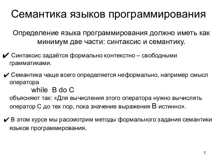 Семантика языков программирования
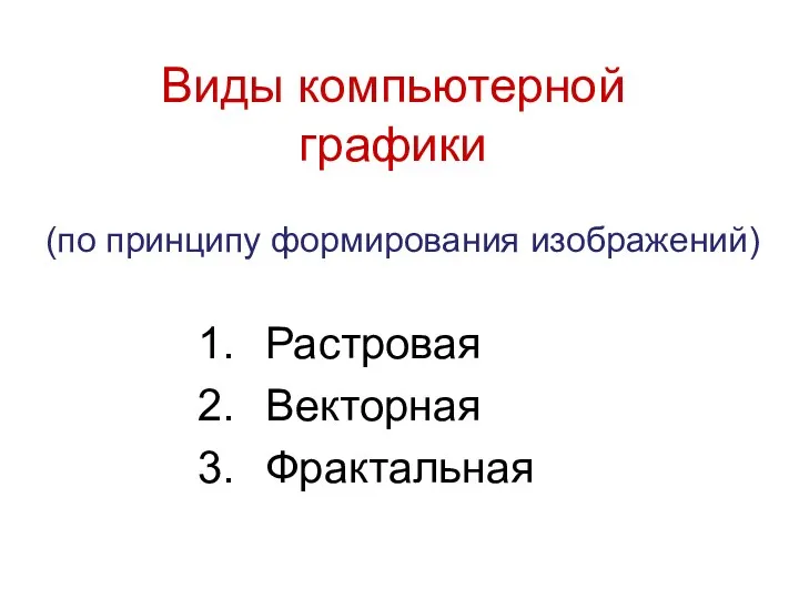 Открытый урок по теме компьютерная графика
 Презантация по информатике Моделирование как метод познания
 С++. История языка Си++
 Системы, модели, графы. Построение информационной модели в виде графа. 8 класс
 Введение в Django
 Логічні операції в мові С
 Основные принципы построения и применения CПО МПС
 Логические величины, операции, выражения
 Графические информационные модели
 База данных в мини-отеле Флёр
 Cтандартные телеграммы при обслуживании рейса
 Організація класів і особливості роботи з об'єктами (тема 12)
 Компьютерные вирусы и антивирусные программы
 Проектирование и реализация дизайн-макета кинотеатра
 Разработка мобильного приложения Квест по УрФУ в дополненной реальности
 Особенности организации защиты информации на предприятии
 Человеко-машинное взаимодействие. XML и QT